
0.5 Solving Equations
In general, equations and inequalities fall into one of three categories: conditional, identity or contradiction, depending on the nature of their solutions. A conditional equation or inequality is true for only certain real numbers. For example, [latex]2x+1 = 7[/latex] is true precisely when [latex]x = 3[/latex], and [latex]w - 3 \leq 4[/latex] is true precisely when [latex]w \leq 7[/latex]. An identity is an equation or inequality that is true for all real numbers. For example, [latex]2x -3 = 1+x-4+x[/latex] or [latex]2t \leq 2t + 3[/latex]. A contradiction is an equation or inequality that is never true. Examples here include [latex]3x - 4 = 3x + 7[/latex] and [latex]a - 1 > a + 3[/latex].
As you may recall, solving an equation or inequality means finding all of the values of the variable, if any exist, which make the given equation or inequality true. This often requires us to manipulate the given equation or inequality from its given form to an easier form. For example, if we’re asked to solve [latex]3 - 2(x-3) = 7x + 3(x+1)[/latex], we get [latex]x = \dfrac{1}{2}[/latex], but not without a fair amount of algebraic manipulation. In order to obtain the correct answer(s), however, we need to make sure that whatever maneuvers we apply are reversible in order to guarantee that we maintain a chain of equivalent equations or inequalities. Two equations or inequalities are called equivalent if they have the same solutions. We summarize these legal moves in the box below.
Procedures which Generate Equivalent Equations
- Add (or subtract) the same real number to (from) both sides of the equation.
- Multiply (or divide) both sides of the equation by the same nonzero real number.[1]
Procedures which Generate Equivalent Inequalities
- Add (or subtract) the same real number to (from) both sides of the equation.
- Multiply (or divide) both sides of the equation by the same positive real number.[2]
0.5.1 Linear Equations
The first equations we wish to review are linear equations as defined below.
An equation is said to be linear in a variable [latex]x[/latex] if it can be written in the form [latex]ax = b[/latex] where [latex]a[/latex] and [latex]b[/latex] are expressions which do not involve [latex]x[/latex] and [latex]a \neq 0[/latex].
One key point about Definition 0.10 is that the exponent on the unknown [latex]x[/latex] in the equation is 1, that is [latex]x = x^1[/latex]. Our main strategy for solving linear equations is summarized below.
Strategy for Solving Linear Equations
In order to solve an equation which is linear in a given variable, says [latex]x[/latex]:
- Isolate all of the terms containing [latex]x[/latex] on one side of the equation, putting all of the terms not containing [latex]x[/latex] on the other side of the equation.
- Factor out the [latex]x[/latex] and divide both sides of the equation by its coefficient.
We illustrate this process with a collection of examples below.
Example 0.5.1
Example 0.5.1.1
Solve the following equations for the indicated variable. Check your answer.
Solve for [latex]x[/latex]: [latex]3x - 6 = 7x + 4[/latex]
Solution:
Solve for [latex]x[/latex]: [latex]3x - 6 = 7x + 4[/latex]
The variable we are asked to solve for is [latex]x[/latex] so our first move is to gather all of the terms involving [latex]x[/latex] on one side and put the remaining terms on the other.[3]
\[ \begin{array}{rclr}
3x – 6 & = & 7x + 4 & \\
(3x-6) – 7x + 6 & = & (7x+4) -7x +6 & \text{Subtract } 7x, \text{ add } 6 \\
3x – 7x – 6 + 6 & = & 7x – 7x + 4 + 6 & \text{Rearrange terms} \\
-4x & = & 10 & 3x-7x = (3-7)x = -4x \\ & & & \\
\dfrac{-4x}{-4} & = & \dfrac{10}{-4} & \text{Divide by the coefficient of } x \\ & & & \\
x & = & -\dfrac{5}{2} & \text{Reduce to lowest terms} \\
\end{array}\]
To check our answer, we substitute [latex]x = -\dfrac{5}{2}[/latex] into each side of the original equation to see the equation is satisfied. Sure enough, [latex]3\left(-\dfrac{5}{2}\right) - 6 = -\dfrac{27}{2}[/latex] and [latex]7\left(-\dfrac{5}{2}\right) + 4 = -\dfrac{27}{2}[/latex].
Example 0.5.1.2
Solve the following equations for the indicated variable. Check your answer.
Solve for [latex]t[/latex]: [latex]3 - 1.7t = \dfrac{t}{4}[/latex]
Solution:
Solve for [latex]t[/latex]: [latex]3 - 1.7t = \dfrac{t}{4}[/latex]
In our next example, the unknown is [latex]t[/latex] and we not only have a fraction but also a decimal to wrangle. Fortunately, with equations we can multiply both sides to rid us of these computational obstacles:
\[ \begin{array}{rclr} 3 – 1.7t & = & \dfrac{t}{4} & \\ & & & \\
40(3 – 1.7t) & = & 40 \left(\dfrac{t}{4}\right) & \text{Multiply by } 40 \\ & & & \\
40(3) – 40(1.7t) & = & \dfrac{40 t}{4} & \text{Distribute} \\
120 – 68t & = & 10 t & \\
(120 -68t) + 68 t & = & 10t + 68 t & \text{Add } 68t \text{ to both sides} \\
120 & = & 78 t & 68t + 10t = (68 + 10)t = 78 t\\
\dfrac{120}{78} & = & \dfrac{78t}{78} & \text{Divide by the coefficient of } t\\ & & & \\
\dfrac{120}{78} & = & t & \\ & & & \\
\dfrac{20}{13} & = & t & \text{Reduce to lowest terms} \\
\end{array}\]
To check, we again substitute [latex]t = \dfrac{20}{13}[/latex] into each side of the original equation.
We find that [latex]3 - 1.7 \left(\dfrac{20}{13}\right) = 3 - \left(\dfrac{17}{10}\right)\left(\dfrac{20}{13}\right) = \dfrac{5}{13}[/latex] and [latex]\dfrac{(20/13)}{4} = \dfrac{20}{13} \cdot \dfrac{1}{4} = \dfrac{5}{13}[/latex] as well.
Example 0.5.1.3
Solve the following equations for the indicated variable. Check your answer.
Solve for [latex]a[/latex]: [latex]\dfrac{1}{18}(7 - 4a) + 2 = \dfrac{a}{3} - \dfrac{4-a}{12}[/latex]
Solution:
Solve for [latex]a[/latex]: [latex]\dfrac{1}{18}(7 - 4a) + 2 = \dfrac{a}{3} - \dfrac{4-a}{12}[/latex]
To solve this next equation, we begin once again by clearing fractions. The least common denominator here is 36:
\[ \begin{array}{rclr}
\dfrac{1}{18}(7 – 4a) + 2 & = & \dfrac{a}{3} – \dfrac{4-a}{12} & \\[8pt]
36 \left(\dfrac{1}{18}(7 – 4a) + 2\right) & = & 36 \left(\dfrac{a}{3} – \dfrac{4-a}{12}\right) & \text{Multiply by } 36\\[13pt]
\dfrac{36}{18} (7-4a) + (36)(2) & = & \dfrac{36a}{3} – \dfrac{36(4-a)}{12} & \text{Distribute} \\[5pt]
2(7-4a) + 72 & = & 12 a – 3(4-a) & \text{Distribute} \\
14 – 8a + 72 & = & 12a – 12 + 3a & \\
86 – 8a & = & 15 a – 12 & 12 a + 3a = (12+3)a = 15 \\
(86-8a)+8a+12 & = & (15a-12) + 8a + 12 & \text{Add } 8a \text{ and }12 \\
86 + 12 – 8a + 8a & = & 15a + 8a – 12 + 12 & \text{Rearrange terms} \\
98 & = & 23 a & 15a + 8a = (15+8)a = 23a \\ & & & \\
\dfrac{98}{23} & = & \dfrac{23a}{23} & \text{Divide by the coefficient of } a \\ & & & \\
\dfrac{98}{23} & = & a &
\end{array} \]
The check, as usual, involves substituting [latex]a = \dfrac{98}{23}[/latex] into both sides of the original equation. The reader is encouraged to work through the (admittedly messy) arithmetic. Both sides work out to [latex]\dfrac{199}{138}[/latex].
Example 0.5.1.4
Solve the following equations for the indicated variable. Check your answer.
Solve for [latex]y[/latex]: [latex]8 y \sqrt{3} + 1 = 7 - \sqrt{12}(5 - y)[/latex]
Solution:
Solve for [latex]y[/latex]: [latex]8 y \sqrt{3} + 1 = 7 - \sqrt{12}(5 - y)[/latex]
The square roots may dishearten you but we treat them just like the real numbers they are. Our strategy is the same: get everything with the variable (in this case [latex]y[/latex]) on one side, put everything else on the other and divide by the coefficient of the variable. We’ve added a few steps to the narrative that we would ordinarily omit just to help you see that this equation is indeed linear.
\[ \begin{array}{rclr}
8 y \sqrt{3} + 1 & = & 7 – \sqrt{12}(5 – y) & \\ & & & \\
8 y \sqrt{3} + 1 & = & 7 – \sqrt{12}(5) + \sqrt{12} y & \text{Distribute} \\ & & & \\
8 y \sqrt{3} + 1 & = & 7 – (2 \sqrt{3})5 + (2 \sqrt{3})y & \sqrt{12} = \sqrt{4\cdot 3} = 2 \sqrt{3} \\ & & & \\
8 y \sqrt{3} + 1 & = & 7 – 10 \sqrt{3} + 2y \sqrt{3} & \\ & & & \\
(8 y \sqrt{3} + 1) – 1 – 2y\sqrt{3} & = & (7 – 10 \sqrt{3} + 2y \sqrt{3}) – 1 – 2y\sqrt{3} & \text{Subtract 1 and } 2y\sqrt{3} \\ & & & \\
8 y \sqrt{3} – 2y\sqrt{3} + 1 – 1 & = & 7 – 1 – 10 \sqrt{3} + 2y \sqrt{3} – 2y\sqrt{3} & \text{Rearrange terms} \\ & & & \\
(8\sqrt{3}-2\sqrt{3})y & = & 6 – 10 \sqrt{3} & \\ & & & \\
6 y \sqrt{3} & = & 6 – 10 \sqrt{3} & \text{See note below} \\ & & & \\
\dfrac{6 y \sqrt{3}}{6 \sqrt{3}} & = & \dfrac{6 – 10 \sqrt{3}}{6 \sqrt{3}} & \text{Divide } 6\sqrt{3} \\ & & & \\
y & = & \dfrac{2 \cdot \sqrt{3} \cdot \sqrt{3} – 2 \cdot 5 \cdot \sqrt{3}}{2 \cdot 3 \cdot \sqrt{3}} & \\ & & & \\
y & = & \dfrac{\cancel{2} \cancel{\sqrt{3}}(\sqrt{3} – 5)}{\cancel{2} \cdot 3 \cdot \cancel{\sqrt{3}}} & \text{Factor and cancel} \\ & & & \\
y & = & \dfrac{\sqrt{3} – 5}{3} & \\
\end{array}\]
In the list of computations above we marked the row [latex]6 y \sqrt{3} = 6 - 10 \sqrt{3}[/latex] with a note. That’s because we wanted to draw your attention to this line without breaking the flow of the manipulations. The equation [latex]6 y \sqrt{3} = 6 - 10 \sqrt{3}[/latex] is in fact linear according to Definition 0.10: the variable is [latex]y[/latex], the value of [latex]A[/latex] is [latex]6\sqrt{3}[/latex] and [latex]B = 6 - 10 \sqrt{3}[/latex]. Checking the solution, while not trivial, is good mental exercise. Each side works out to be [latex]\dfrac{27 - 40 \sqrt{3}}{3}[/latex].
Example 0.5.1.5
Solve the following equations for the indicated variable. Check your answer.
Solve for [latex]x[/latex]: [latex]\dfrac{3x-1}{2} = x\sqrt{50} + 4[/latex]
Solution:
Solve for [latex]x[/latex]: [latex]\dfrac{3x-1}{2} = x\sqrt{50} + 4[/latex]
Proceeding as before, we simplify radicals and clear denominators. Once we gather all of the terms containing [latex]x[/latex] on one side and move the other terms to the other, we factor out [latex]x[/latex] to identify its coefficient then divide to get our answer.
\[ \begin{array}{rclr}
\dfrac{3x-1}{2} & = & x\sqrt{50} + 4 & \\ & & & \\
\dfrac{3x-1}{2} & = & 5x\sqrt{2} + 4 & \sqrt{50} = \sqrt{25 \cdot 2} \\ & & & \\
2\left(\dfrac{3x-1}{2}\right) & = & 2 \left(5x\sqrt{2} + 4 \right) & \text{Multiply by 2} \\ & & & \\
\dfrac{\cancel{2} \cdot (3x-1)}{\cancel{2}} & = & 2 (5x \sqrt{2}) + 2\cdot 4 & \text{Distribute} \\ & & & \\
3x – 1 & = & 10x \sqrt{2} + 8 & \\
(3x-1) – 10x\sqrt{2} + 1 & = & (10x \sqrt{2} + 8) – 10x\sqrt{2} + 1 & \text{Subtract } 10x\sqrt{2}, \text{ add 1} \\
3x – 10x\sqrt{2} – 1 + 1 & = & 10x\sqrt{2} – 10x\sqrt{2} + 8 + 1 & \text{Rearrange terms} \\
3x – 10x\sqrt{2} & = & 9 & \\
(3 – 10\sqrt{2}) x & = & 9 & \text{Factor} \\ & & & \\
\dfrac{(3 – 10\sqrt{2}) x}{3 – 10\sqrt{2}} & = & \dfrac{9}{3 – 10\sqrt{2}} & \text{Divide by the coefficient of } x \\ & & & \\
x & = & \dfrac{9}{3 – 10\sqrt{2}} & \\
\end{array} \]
The reader is encouraged to check this solution – it isn’t as bad as it looks if you’re careful! Each side works out to be [latex]\dfrac{12 + 5\sqrt{2}}{3-10\sqrt{2}}[/latex].
Example 0.5.1.6
Solve the following equations for the indicated variable. Check your answer.
Solve for [latex]y[/latex]: [latex]x(4-y) = 8y[/latex]
Solution:
Solve for [latex]y[/latex]: [latex]x(4-y) = 8y[/latex]
If we were instructed to solve our last equation for [latex]x[/latex], we’d be done in one step: divide both sides by [latex](4-y)[/latex] – assuming [latex]4-y \neq 0[/latex], that is. Alas, we are instructed to solve for [latex]y[/latex], which means we have some more work to do.
\[ \begin{array}{rclr}
x(4-y) & = & 8y & \\
4x – xy & = & 8y & \text{Distribute} \\
(4x – xy) + xy & = & 8y + xy & \text{Add } xy \\
4x & = & (8+x)y & \text{Factor} \\
\end{array}\]
In order to finish the problem, we need to divide both sides of the equation by the coefficient of [latex]y[/latex] which in this case is [latex]8+x[/latex]. This expression contains a variable so we need to stipulate that we may perform this division only if [latex]8 + x \neq 0[/latex], or, in other words, [latex]x \neq -8[/latex]. Hence, we write our solution as:\[ y = \dfrac{4x}{8+x}, \quad \text{provided } x \neq -8\] What happens if [latex]x = -8[/latex]? Substituting [latex]x = -8[/latex] into the original equation gives [latex](-8)(4-y) = 8y[/latex] or [latex]-32 + 8y = 8y[/latex]. This reduces to [latex]-32 = 0[/latex], which is a contradiction. This means there is no solution when [latex]x = -8[/latex], so we’ve covered all the bases. Checking our answer requires some Algebra we haven’t reviewed yet in this text, but the necessary skills should be lurking somewhere in the mathematical mists of your mind. The adventurous reader is invited to plug [latex]y = \dfrac{4x}{8 + x}[/latex] into the original equation and show that both sides work out to [latex]\dfrac{32x}{x + 8}[/latex].
0.5.2 Absolute Value Equations
In this subsection, we review some of the basic concepts involving the absolute value of a real number [latex]x[/latex]. There are a few different ways to define absolute value and in this section we choose the following definition. (Absolute value will be revisited in much greater depth in Section 1.4 where we present what one can think of as the “precise” definition.)
Definition 0.11 Absolute Value as Distance
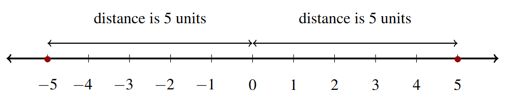
For every real number [latex]x[/latex], the absolute value of [latex]x[/latex], denoted [latex]|x|[/latex], is the distance between [latex]x[/latex] and 0 on the number line. More generally, if [latex]x[/latex] and [latex]c[/latex] are real numbers, [latex]|x-c|[/latex] is the distance between the numbers [latex]x[/latex] and [latex]c[/latex]on the number line.
For example, [latex]|5| = 5[/latex] and [latex]|-5| = 5[/latex], because each is 5 units from 0 on the number line:
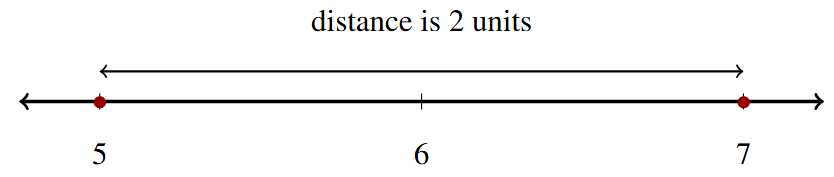
Computationally, the absolute value makes negative numbers positive, though we need to be a little cautious with this description. While [latex]|-7| = 7[/latex], [latex]|5-7| \neq 5+7[/latex]. The absolute value acts as a grouping symbol, so [latex]|5-7| = |-2| = 2[/latex], which makes sense as 5 and 7 are two units away from each other on the number line:
Next, we list some of the operational properties of absolute value.
Let [latex]a[/latex] and [latex]b[/latex] be real numbers and let [latex]n[/latex] be an integer.[4]
- Product Rule: [latex]|ab|= |a||b|[/latex]
- Power Rule: [latex]\left| a^{n} \right| = |a|^{n}[/latex] whenever [latex]a^{n}[/latex] is defined
- Quotient Rule: [latex]\left| \dfrac{a}{b} \right| = \dfrac{|a|}{|b|}[/latex], provided [latex]b \neq 0[/latex]
The proof of Theorem 0.3 is difficult, but not impossible, using the distance definition of absolute value or even the it makes negatives positive notion. It is, however, much easier if one uses the “precise” definition given in Section 1.4 so we will revisit the proof then. For now, let’s focus on how to solve basic equations and inequalities involving the absolute value.
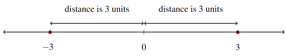
Thinking of absolute value in terms of distance gives us a geometric way to interpret equations. For example, to solve [latex]|x| = 3[/latex], we are looking for all real numbers [latex]x[/latex] whose distance from 0 is 3 units. If we move three units to the right of 0, we end up at [latex]x = 3[/latex]. If we move three units to the left, we end up at [latex]x = -3[/latex]. Thus the solutions to [latex]|x| = 3[/latex] are [latex]x = \pm 3[/latex].
Thinking this way gives us the following.
Suppose [latex]x[/latex], [latex]y[/latex] and [latex]c[/latex] are real numbers.
- [latex]|x| = 0[/latex] if and only if [latex]x = 0[/latex].
- For [latex]c > 0[/latex], [latex]|x| = c[/latex] if and only if [latex]x = c[/latex] or [latex]x = -c[/latex].
- For [latex]c[/latex]< 0, [latex]|x| = c[/latex] has no solution.
- [latex]|x| = |y|[/latex] if and only if [latex]x = y[/latex] or [latex]x = -y[/latex].
(That is, if two numbers have the same absolute values, they are either the same number or exact opposites of each other.)
Theorem 0.4 is our main tool in solving equations involving the absolute value, as it allows us a way to rewrite such equations as compound linear equations.
Strategy for Solving Equations Involving Absolute Value
In order to solve an equation involving the absolute value of a quantity [latex]|X|[/latex]:
- Isolate the absolute value on one side of the equation so it has the form [latex]|X| = c[/latex].
- Apply Theorem 0.4.
The techniques we use to isolate the absolute value are precisely those we used in the previous subsection to isolate the variable when solving linear equations. Time for some practice.
Example 0.5.2
Example 0.5.2.1
Solve each of the following equations.
[latex]|3x-1| = 6[/latex]
Solution:
Solve the equation: [latex]|3x-1| = 6[/latex].
The equation [latex]|3x-1| = 6[/latex] is of already in the form [latex]|X| = c[/latex], so we know that either [latex]3x-1=6[/latex] or [latex]3x-1 = -6[/latex]
Solving the equation [latex]3x-1=6[/latex] gives us [latex]x = \dfrac{7}{3}[/latex].
While solving the equation [latex]3x-1 = -6[/latex] yields [latex]x = -\dfrac{5}{3}[/latex].
We may check both of these solutions by substituting them into the original equation and showing that the arithmetic works out.
Example 0.5.2.2
Solve each of the following equations.
[latex]\dfrac{3 - |y+5|}{2} = 1[/latex]
Solution:
Solve the equation: [latex]\dfrac{3 - |y+5|}{2} = 1[/latex].
We begin solving [latex]\dfrac{3 - |y+5|}{2} = 1[/latex] by isolating the absolute value to put it in the form [latex]|X| = c[/latex].
\[ \begin{array}{rclr}
\dfrac{3 – |y+5|}{2} & = & 1 & \\
3 – |y+5| & = & 2 & \text{Multiply by } 2\\
-|y+5| & = & -1 & \text{Subtract } 3 \\
|y+5| & = & 1 & \text{Divide by } -1 \\
\end{array} \]
At this point, we have [latex]y+5 = 1[/latex] or [latex]y+5 = -1[/latex], so our solutions are [latex]y = -4[/latex] or [latex]y = -6[/latex].
We leave it to the reader to check both answers in the original equation.
Example 0.5.2.3
Solve each of the following equations.
[latex]3|2t+1| - \sqrt{5} = 0[/latex]
Solution:
Solve the equation: [latex]3|2t+1| - \sqrt{5} = 0[/latex].
As in the previous example, we first isolate the absolute value. Don’t let the [latex]\sqrt{5}[/latex] throw you off – it’s just another real number, so we treat it as such:
\[ \begin{array}{rclr}
3|2t+1| – \sqrt{5} & = & 0 & \\
3|2t+1| & = & \sqrt{5} & \text{Add }\sqrt{5} \\
|2t + 1| & = & \dfrac{\sqrt{5}}{3} & \text{Divide by } 3\\
\end{array} \]
From here, we have that [latex]2t+1 = \dfrac{\sqrt{5}}{3}[/latex] or [latex]2t+1 = -\dfrac{\sqrt{5}}{3}[/latex].
The first equation gives [latex]t = \dfrac{\sqrt{5}-3}{6}[/latex] while the second gives [latex]t = \dfrac{-\sqrt{5}-3}{6}[/latex] thus we list our answers as [latex]t = \dfrac{-3 \pm \sqrt{5}}{6}[/latex].
The reader should enjoy the challenge of substituting both answers into the original equation and following through the arithmetic to see that both answers work.
Example 0.5.2.4
Solve each of the following equations.
[latex]4 - |5w+3| = 5[/latex]
Solution:
Solve the equation: [latex]4 - |5w+3| = 5[/latex].
Upon isolating the absolute value in the equation [latex]4 - |5w+3| = 5[/latex], we get [latex]|5w+3| = -1[/latex].
At this point, we know there cannot be any real solution. By definition, the absolute value is a distance, and as such is never negative. We write “no solution” and carry on.
Example 0.5.2.5
Solve each of the following equations.
[latex]\left|3 - x \sqrt[3]{12}\right| = |4x+1|[/latex]
Solution:
Solve the equation: [latex]\left|3 - x \sqrt[3]{12}\right| = |4x+1|[/latex].
Our next equation already has the absolute value expressions (plural) isolated, so we work from the principle that if [latex]|x| = |y|[/latex], then [latex]x = y[/latex] or [latex]x = -y[/latex].
Thus from [latex]\left|3 - x \sqrt[3]{12}\right| = |4x+1|[/latex] we get two equations to solve: \[ 3 – x \sqrt[3]{12} = 4x+1, \qquad \text{and} \qquad 3 – x \sqrt[3]{12} = -(4x+1) \]
Notice that the right side of the second equation is [latex]-(4x+1)[/latex] and not simply [latex]-4x+1[/latex]. Remember, the expression [latex]4x+1[/latex] represents a single real number so in order to negate it we need to negate the entire expression [latex]-(4x+1)[/latex].
Moving along, when solving [latex]3 - x \sqrt[3]{12} = 4x+1[/latex], we obtain [latex]x = \dfrac{2}{4 + \sqrt[3]{12}}[/latex].
The solution to [latex]3 - x \sqrt[3]{12} = -(4x+1)[/latex] is [latex]x = \dfrac{4}{\sqrt[3]{12}-4}[/latex].
As usual, the reader is invited to check these answers by substituting them into the original equation.
Example 0.5.2.6
Solve each of the following equations.
[latex]|t-1| - 3|t+1| = 0[/latex]
Solution:
Solve the equation: [latex]|t-1| - 3|t+1| = 0[/latex].
We start by isolating one of the absolute value expressions: [latex]|t-1| - 3|t+1| = 0[/latex] gives [latex]|t-1| = 3|t+1|[/latex].
While this resembles the form [latex]|x| = |y|[/latex], the coefficient 3 in [latex]3|t+1|[/latex] prevents it from being an exact match. Not to worry – because 3 is positive, [latex]3 = |3|[/latex] so \[3|t+1| = |3| |t+1| = |3(t+1)| = |3t+3|.\]
Hence, our equation becomes [latex]|t-1| = |3t+3|[/latex] which results in the two equations: [latex]t-1 = 3t+3[/latex] and [latex]t-1 = -(3t+3)[/latex].
The first equation gives [latex]t = -2[/latex] and the second gives [latex]t = -\dfrac{1}{2}[/latex].
The reader is encouraged to check both answers in the original equation.
0.5.3 Solving Equations By Factoring
Many students wonder why they are forced to learn how to factor. Simply put, factoring is our main tool for solving the non-linear equations which arise in many of the applications of Mathematics.[5] We use factoring in conjunction with the Zero Product Property of Real Numbers which was first stated in Section 0.1 and is given here again for reference.
Zero Product Property of Real Numbers
If [latex]a[/latex] and [latex]b[/latex] are real numbers with [latex]ab = 0[/latex] then either [latex]a = 0[/latex] or [latex]b = 0[/latex] or both.
Consider the equation [latex]6x^2 + 11x = 10[/latex]. To see how the Zero Product Property is used to help us solve this equation, we first set the equation equal to zero and then apply the techniques from Example 0.3.2:
\[ \begin{array}{rclr}
6x^2 + 11x & = & 10 \\
6x^2 + 11x – 10 & = & 0 & \text{Subtract 10 from both sides} \\
(2x+5)(3x-2) & = & 0 & \text{Factor} \\
2x +5 = 0 & \text{or} & 3x -2 = 0 & \text{Zero Product Property} \\
& & & a = 2x+5, b = 3x-2 \\
x = -\dfrac{5}{2} & \text{or} & x = \dfrac{2}{3} & \\
\end{array} \]
The reader should check that both of these solutions satisfy the original equation.
It is critical that you see the importance of setting the expression equal to 0 before factoring. Otherwise, we’d get something silly like:
\[ \begin{array}{rclr}
6x^2 + 11x & = & 10 \\
x(6x + 11) & = & 10 & \text{Factor} \\
\end{array} \]
We summarize the correct equation solving strategy below.
Strategy for Solving Non-linear Equations
- Put all of the nonzero terms on one side of the equation so that the other side is 0.
- Factor.
- Use the Zero Product Property of Real Numbers and set each factor equal to 0.
- Solve each of the resulting equations.
Let’s finish the subsection with a collection of examples in which we use this strategy.
Example 0.5.3
Example 0.5.3.1
Solve each of the following equations.
[latex]3x^2 = 35 - 16x[/latex]
Solution:
Solve the equation: [latex]x^2 = 35 - 16x[/latex].
We begin by gathering all of the nonzero terms to one side getting 0 on the other. Then we proceed to factor and apply the Zero Product Property.
\[ \begin{array}{rclr}
3x^2 & = & 35 – 16x & \\
3x^2 + 16x – 35 & = & 0 & \text{Add } 16x, \text{ subtract } 35 \\
(3x-5)(x+7) & = & 0 & \text{Factor} \\
3x-5 = 0 & \text{or} & x+7 = 0 & \text{Zero Product Property} \\
x = \dfrac{5}{3} & \text{or} & x = -7 & \\
\end{array} \]
We check our answers by substituting each of them into the original equation. Plugging in [latex]x = \dfrac{5}{3}[/latex] yields [latex]\dfrac{25}{3}[/latex] on both sides while [latex]x = -7[/latex] gives 147 on both sides.
Example 0.5.3.2
Solve each of the following equations.
[latex]t = \dfrac{1+4t^2}{4}[/latex]
Solution:
Solve the equation: [latex]t = \dfrac{1+4t^2}{4}[/latex].
To solve [latex]t = \dfrac{1+4t^2}{4}[/latex], we first clear fractions. Then move all of the nonzero terms to one side of the equation, factor and apply the Zero Product Property.
\[ \begin{array}{rclr}
t & = & \dfrac{1+4t^2}{4} & \\
4t & = & 1+4t^2 & \text{Clear fractions (multiply by 4)} \\
0 & = & 1+4t^2 – 4t & \text{Subtract 4} \\
0 & = & 4t^2 – 4t + 1 & \text{Rearrange terms} \\
0 & = & (2t-1)^2 & \text{Factor (Perfect Square Trinomial)} \\
\end{array} \]
At this point, we get [latex](2t-1)^2 = (2t-1)(2t-1) = 0[/latex], so, the Zero Product Property gives us [latex]2t-1 =0[/latex] in both cases.[6]
Our final answer is [latex]t = \dfrac{1}{2}[/latex], which we invite the reader to check.
Example 0.5.3.3
Solve each of the following equations.
[latex](y-1)^2 = 2(y-1)[/latex]
Solution:
Solve the equation: [latex](y-1)^2 = 2(y-1)[/latex].
Following the strategy outlined above, the first step to solving [latex](y-1)^2 = 2(y-1)[/latex] is to gather the nonzero terms on one side of the equation with 0 on the other side and factor.
\[ \begin{array}{rclr}
(y-1)^2 & = & 2(y-1) & \\
(y-1)^2 – 2(y-1) & = & 0 & \text{Subtract } 2(y-1) \\
(y-1)[(y-1) – 2] & = & 0 & \text{Factor out G.C.F.} \\
(y-1)(y-3) & = & 0 & \text{Simplify} \\
y-1 = 0 & \text{or} & y – 3 = 0 & \\
y = 1 & \text{or} & y = 3 & \\
\end{array} \]
Both of these answers are easily checked by substituting them into the original equation.
An alternative method to solving this equation is to begin by dividing both sides by [latex](y-1)[/latex] to simplify things outright. As we saw in Example 0.5.1, however, whenever we divide by a variable quantity, we make the explicit assumption that this quantity is nonzero. Thus we must stipulate that [latex]y - 1 \neq 0[/latex].
\[ \begin{array}{rclr}
\dfrac{(y-1)^2}{(y-1)} & = & \dfrac{2(y-1)}{(y-1)} & \text{Divide by } (y-1) \text{ – this assumes } (y-1) \neq 0\\
y – 1 & = & 2 & \\
y & = & 3 & \\
\end{array} \]
Note that in this approach, we obtain the [latex]y=3[/latex] solution, but we lose the [latex]y = 1[/latex] solution. How did that happen? Assuming [latex]y - 1 \neq 0[/latex] is equivalent to assuming [latex]y \neq 1[/latex]. This is an issue because [latex]y = 1[/latex] is a solution to the original equation and it was divided out too early. The moral of the story? If you decide to divide by a variable expression, double check that you aren’t excluding any solutions.[7]
Example 0.5.3.4
Solve each of the following equations.
[latex]\dfrac{w^4}{3} = \dfrac{8w^3-12}{12} - \dfrac{w^2-4}{4}[/latex]
Solution:
Solve the equation: [latex]\dfrac{w^4}{3} = \dfrac{8w^3-12}{12} - \dfrac{w^2-4}{4}[/latex].
Proceeding as before, we clear fractions, gather the nonzero terms on one side of the equation, have 0 on the other and factor.
\[ \begin{array}{rclr}
\dfrac{w^4}{3} & = & \dfrac{8w^3-12}{12} – \dfrac{w^2-4}{4} & \\ & & & \\
12 \left(\dfrac{w^4}{3}\right) & = & 12 \left(\dfrac{8w^3-12}{12} – \dfrac{w^2-4}{4} \right) & \text{Multiply by 12}\\ & & & \\
4w^4 & = & (8w^3 – 12) – 3(w^2-4) & \text{Distribute} \\
4w^4 & = & 8w^3 – 12 – 3w^2 + 12 & \text{Distribute} \\
0 & = & 8w^3 – 12 – 3w^2 + 12 – 4w^4 & \text{Subtract } 4w^4 \\
0 & = & 8w^3 – 3w^2 – 4w^4 & \text{Gather like terms} \\
0 & = & w^2(8w – 3 – 4w^2) & \text{Factor out G.C.F.} \\
\end{array} \]
At this point, we apply the Zero Product Property to deduce that [latex]w^2 = 0[/latex] or [latex]8w - 3 - 4w^2 = 0[/latex].
From [latex]w^2 = 0[/latex], we get [latex]w = 0[/latex].
To solve [latex]8w - 3 - 4w^2 = 0[/latex], we rearrange terms and factor:
\[-4w^2 + 8w – 3= (2w – 1)(-2w+3) = 0.\]
Applying the Zero Product Property again, we get [latex]2w - 1= 0[/latex] (which gives [latex]w = \dfrac{1}{2}[/latex]),
or [latex]-2w+3 = 0[/latex] (which gives [latex]w = \dfrac{3}{2}[/latex]).
Our final answers are [latex]w = 0[/latex], [latex]w = \dfrac{1}{2}[/latex] and [latex]w = \dfrac{3}{2}[/latex].
The reader is encouraged to check each of these answers in the original equation. (You need the practice with fractions!)
Example 0.5.3.5
Solve each of the following equations.
[latex]z(z(18z+9)-50) = 25[/latex]
Solution:
Solve the equation: [latex]z(z(18z+9)-50) = 25[/latex].
For our next example, we begin by subtracting the 25 from both sides then work out the indicated operations before factoring by grouping.
\[ \begin{array}{rclr}
z(z(18z+9)-50) & = & 25 & \\
z(z(18z+9)-50) – 25 & = & 0 & \text{Subtract 25} \\
z(18z^2 + 9z – 50) – 25 & = & 0 & \text{Distribute} \\
18z^3 + 9z^2 – 50z – 25 & = & 0 & \text{Distribute} \\
9z^2(2z + 1) – 25(2z + 1) & = & 0 & \text{Factor} \\
(9z^2 – 25)(2z+1) & = & 0 & \text{Factor} \\
\end{array} \]
At this point, we use the Zero Product Property and get [latex]9z^2 - 25 = 0[/latex] or [latex]2z + 1 = 0[/latex].
The latter gives [latex]z = -\dfrac{1}{2}[/latex] whereas the former factors as [latex](3z - 5)(3z+5) = 0[/latex].
Applying the Zero Product Property again gives [latex]3z-5 = 0[/latex] (so [latex]z = \dfrac{5}{3}[/latex])
or [latex]3z+5 = 0[/latex] (so [latex]z = -\dfrac{5}{3}[/latex].)
Our final answers are [latex]z = -\dfrac{1}{2}[/latex], [latex]z = \dfrac{5}{3}[/latex] and [latex]z = -\dfrac{5}{3}[/latex], each of which is good fun to check.
Example 0.5.3.6
Solve each of the following equations.
[latex]x^4-8x^2 - 9 = 0[/latex]
Solution:
Solve the equation: [latex]x^4-8x^2 - 9 = 0[/latex].
The nonzero terms of the equation [latex]x^4-8x^2 - 9= 0[/latex] are already on one side of the equation so we proceed to factor.
This trinomial doesn’t fit the pattern of a perfect square so we attempt to reverse the F.O.I.L.ing process. With an [latex]x^4[/latex] term, we have two possible forms to try: [latex](ax^2 + b)(cx^2 + d)[/latex] and [latex](ax^3 + b)(cx +d)[/latex]. We leave it to you to show that [latex](ax^3 + b)(cx +d)[/latex] does not work and we show that [latex](ax^2 + b)(cx^2 + d)[/latex]does.
Due to the fact that the coefficient of [latex]x^4[/latex] is 1, we take [latex]a = c = 1[/latex].
The constant term is [latex]-9[/latex] so we know [latex]b[/latex] and [latex]d[/latex] have opposite signs and our choices are limited to two options: either [latex]b[/latex] and [latex]d[/latex] come from [latex]\pm 1[/latex] and [latex]\mp 9[/latex] OR one is 3 while the other is [latex]-3[/latex].
After some trial and error, we get [latex]x^4 - 8x^2 - 9 = (x^2 - 9)(x^2+1)[/latex].
Hence the equation [latex]x^4-8x^2 - 9= 0[/latex] may be rewritten as [latex](x^2 - 9)(x^2 + 1) = 0[/latex].
The Zero Product Property tells us that either [latex]x^2 - 9 = 0[/latex] or [latex]x^2+1 = 0.[/latex]
To solve [latex]x^2 - 9 = 0[/latex]
we factor: [latex](x-3)(x+3) = 0[/latex],
so [latex]x-3 = 0[/latex] or [latex]x+3 = 0[/latex],
so [latex]x=3[/latex] or [latex]x = -3[/latex].
The equation [latex]x^2 + 1 = 0[/latex] has no (real) solution, because for any real number [latex]x[/latex], [latex]x^2[/latex] is always 0 or greater. Thus [latex]x^2 + 1[/latex] is always positive.
Our final answers are [latex]x = 3[/latex] and [latex]x = -3[/latex].
As always, the reader is invited to check both answers in the original equation.
0.5.4 Solving Radical Equations
Theorem 0.2 allows us to generalize the process of Extracting Square Roots to Extracting nth Roots which in turn allows us to solve equations[8] of the form [latex]X^n = c[/latex].
- If [latex]c[/latex] is a real number and [latex]n[/latex] is odd then the real number solution to [latex]X^{n} = c[/latex] is [latex]X = \sqrt[n]{c}[/latex].
- If [latex]c \geq 0[/latex] and [latex]n[/latex] is even then the real number solutions to [latex]X^{n} = c[/latex] are [latex]X = \pm \sqrt[n]{c}[/latex].
Note: If [latex]c 0[/latex] and [latex]n[/latex] is even then [latex]X^{n} = c[/latex] has no real number solutions.
Essentially, we solve [latex]X^{n} = c[/latex] by taking the nth root’ of both sides: [latex]\sqrt[n]{X^{n}} = \sqrt[n]{c}[/latex]. Simplifying the left side gives us just [latex]X[/latex] if [latex]n[/latex] is odd or [latex]|X|[/latex] if [latex]n[/latex] is even. In the first case, [latex]X = \sqrt[n]{c}[/latex], and in the second, [latex]X = \pm \sqrt[n]{c}[/latex].
Putting this together with the other part of Theorem 0.2, namely [latex](\sqrt[n]{a})^n = a[/latex], gives us a strategy for solving equations which involve nth powers and nth roots.
Strategies for Solving Power and Radical Equations
- If the equation involves an nth power and the variable appears in only one term, isolate the term with the nth power and extract nth roots.
- If the equation involves an nth root and the variable appears in that nth root, isolate the nth root and raise both sides of the equation to the nth power.
Note: When raising both sides of an equation to an even power, be sure to check for extraneous solutions.
The note about extraneous solutions can be demonstrated by the basic equation: [latex]\sqrt{x} = -2[/latex]. This equation has no solution because, by definition, [latex]\sqrt{x} \geq 0[/latex] for all real numbers [latex]x[/latex]. However, if we square both sides of this equation, we get [latex](\sqrt{x})^2 = (-2)^2[/latex] or [latex]x = 4[/latex]. However, [latex]x = 4[/latex] doesn’t check in the original equation, as [latex]\sqrt{4} = 2[/latex], not [latex]-2[/latex]. Once again, the root[9] of all of our problems lies in the fact that a negative number to an even power results in a positive number. In other words, raising both sides of an equation to an even power does not produce an equivalent equation, but rather, an equation which may possess more solutions than the original. Hence the cautionary remark above about extraneous solutions.
Example 0.5.4
Example 0.5.4.1
Solve each of the following equations.
[latex](5x +3)^{4} = 16[/latex]
Solution:
Solve the equation: [latex](5x +3)^{4} = 16[/latex].
In our first equation, the quantity containing [latex]x[/latex] is already isolated, so we extract fourth roots. The exponent is even, so when the roots are extracted we need both the positive and negative roots
\[ \begin{array}{rclr}
(5x +3)^{4} & = & 16 & \\ & & & \\
5x+3 & = & \pm \sqrt[4]{16} & \text{Extract fourth roots} \\ & & &\\
5x + 3 & = & \pm 2 & \\ & & & \\
5x+3 = 2 & \text{or} & 5x+3 = -2 & \\
x = -\dfrac{1}{5} & \text{or} & x = -1 \\
\end{array} \]
We leave it to the reader to verify that both of these solutions satisfy the original equation.
Example 0.5.4.2
Solve each of the following equations.
[latex]1 - \dfrac{(5-2w)^3}{7} = 9[/latex]
Solution:
Solve the equation: [latex]1 - \dfrac{(5-2w)^3}{7} = 9[/latex].
In this example, we first need to isolate the quantity containing the variable [latex]w[/latex]. Here, third (cube) roots are required and the exponent (index) is odd indicating we do not need the [latex]\pm[/latex]:
\[ \begin{array}{rclr}
1 – \dfrac{(5-2w)^3}{7} & = & 9 & \\ & & &\\
– \dfrac{(5-2w)^3}{7} & = & 8 & \text{Subtract } 1\\ & & &\\
(5-2w) ^ 3 & = & -56 & \text{Multiply by } -7 \\ & & &\\
5 – 2w & = & \sqrt[3]{-56} & \text{Extract cube root} \\
5 – 2w & = & \sqrt[3]{(-8)(7)} & \\
5 – 2w & = & \sqrt[3]{-8} \sqrt[3]{7} & \text{Product Rule}\\ & & &\\
5 – 2w & = & -2\sqrt[3]{7} & \\ & & &\\
-2w & = & -5-2 \sqrt[3]{7} & \text{Subtract } 5 \\ & & &\\
w & = & \dfrac{-5 – 2\sqrt[3]{7}}{-2} & \text{Divide by } -2 \\ & & &\\
w & = & \dfrac{5 + 2\sqrt[3]{7}}{2} & \text{Properties of Negatives}
\end{array}\]
The reader should check the answer because it provides a hearty review of arithmetic.
Example 0.5.4.3
Solve each of the following equations.
[latex]t + \sqrt{2t+3} = 6[/latex]
Solution:
Solve the equation: [latex]t + \sqrt{2t+3} = 6[/latex].
To solve [latex]t + \sqrt{2t+3} = 6[/latex], we first isolate the square root, then proceed to square both sides of the equation. In doing so, we run the risk of introducing extraneous solutions therefore checking our answers here is a necessity.
\[ \begin{array}{rclr}
t + \sqrt{2t+3} & = & 6 & \\ & & &\\
\sqrt{2t+3} & = & 6 – t & \text{Subtract } t \\ & & &\\
(\sqrt{2t+3})^2 & = & (6-t)^2 & \text{Square both sides} \\ & & &\\
2t + 3 & = & 36-12t + t^2 & \text{F.O.I.L. / Perfect Square Trinomial} \\ & & &\\
0 & = & t^2 – 14t + 33 & \text{Subtract } 2t \text{ and } 3 \\ & & &\\
0 & = & (t-3)(t-11) & \text{Factor} \\
\end{array} \]
From the Zero Product Property, we know either [latex]t - 3 = 0[/latex] (which gives [latex]t=3[/latex]) or [latex]t-11 = 0[/latex] (which gives [latex]t=11[/latex]).
When checking our answers, we find [latex]t = 3[/latex] satisfies the original equation, but [latex]t = 11[/latex] does not.
It is worth noting that when [latex]t=11[/latex] is substituted into the original equation, we get [latex]11 + \sqrt{25} = 6[/latex]. If the [latex]+\sqrt{25}[/latex] were [latex]-\sqrt{25}[/latex], the solution would check.
Once again, when squaring both sides of an equation, we lose track of [latex]\pm[/latex], which is what lets extraneous solutions in the door.
So our final answer is [latex]t = 3[/latex] only.
Example 0.5.4.4
Solve each of the following equations.
[latex]\sqrt{2} - 3\sqrt[3]{2y+1} = 0[/latex]
Solution:
Solve the equation: [latex]\sqrt{2} - 3\sqrt[3]{2y+1} = 0[/latex].
In our next example, we locate the variable (in this case [latex]y[/latex]) beneath a cube root, so we first isolate that root and cube both sides.
\[ \begin{array}{rclr}
\sqrt{2} – 3\sqrt[3]{2y+1} & = & 0 & \\ & & &\\
– 3\sqrt[3]{2y+1} & = & – \sqrt{2} & \text{Subtract } \sqrt{2} \\ & & &\\
\sqrt[3]{2y+1} & = & \dfrac{-\sqrt{2}}{-3} & \text{Divide by } -3 \\
\sqrt[3]{2y+1} & = & \dfrac{\sqrt{2}}{3} & \text{Properties of Negatives} \\& & &\\
(\sqrt[3]{2y+1})^3 & = & \left( \dfrac{\sqrt{2}}{3} \right)^{3} & \text{Cube both sides} \\ & & &\\
2y + 1 & = & \dfrac{(\sqrt{2})^3}{3^3} & \\& & &\\
2y + 1 & = & \dfrac{2\sqrt{2}}{27} & \\ [& & &\\
2y & = & \dfrac{2 \sqrt{2}}{27} – 1 & \text{Subtract } 1 \\[8pt]
2y & = & \dfrac{2 \sqrt{2}}{27} – \dfrac{27}{27} & \text{Common denominators} \\ & & &\\
2y & = & \dfrac{2 \sqrt{2} – 27}{27} & \text{Subtract fractions} \\ & & &\\
y & = & \dfrac{2 \sqrt{2} – 27}{54} & \text{Divide by } \left(\text{multiply by } \dfrac{1}{2} \right) \\
\end{array}\]
As we raised both sides to an odd power, we don’t need to worry about extraneous solutions but we encourage the reader to check the solution just for the fun of it.
Example 0.5.4.5
Solve each of the following equations.
[latex]\sqrt{4x-1} + 2\sqrt{1 - 2x} = 1[/latex]
Solution:
Solve the equation: [latex]\sqrt{4x-1} + 2\sqrt{1 - 2x} = 1[/latex].
In the equation [latex]\sqrt{4x-1} + 2\sqrt{1 - 2x} = 1[/latex], we have not one but two square roots. We begin by isolating one of the square roots and squaring both sides.
\[ \begin{array}{rclr}
\sqrt{4x-1} + 2\sqrt{1 – 2x} & = & 1 & \\ & & &\\
\sqrt{4x-1} & = & 1 – 2\sqrt{1-2x} & \text{Subtract } 2\sqrt{1 – 2x} \text{ from both sides} \\ & & &\\
(\sqrt{4x-1})^2 & = & (1 – 2\sqrt{1-2x})^2 & \text{Square both sides} \\ & & &\\
4x – 1 & = & 1 – 4\sqrt{1-2x} + (2\sqrt{1-2x})^2 & \text{F.O.I.L. / Perfect Square Trinomial} \\ & & &\\
4x – 1 & = & 1 – 4\sqrt{1-2x} + 4(1-2x) & \\ & & &\\
4x – 1 & = & 1 – 4\sqrt{1-2x} + 4 – 8x & \text{Distribute} \\ & & &\\
4x – 1 & = & 5 – 8x – 4\sqrt{1-2x} & \text{Gather like terms} \\
\end{array} \]
At this point, we have just one square root so we proceed to isolate it and square both sides a second time.[10]
\[ \begin{array}{rclr}
4x – 1 & = & 5 – 8x – 4\sqrt{1-2x} & \\ & & &\\
12x – 6 & = & -4\sqrt{1-2x} & \text{Subtract 5, add } 8x\\ & & &\\
(12x-6)^2 & = & (-4\sqrt{1-2x})^2 & \text{Square both sides} \\ & & &\\
144x^2 – 144x + 36 & = & 16(1-2x) & \\ & & &\\
144x^2 – 144x + 36 & = & 16 – 32x & \\ & & &\\
144x^2 – 112x + 20 & = & 0 & \text{Subtract 16, add } 32x \\ & & &\\
4(36x^2 – 28x + 5) & = & 0 & \text{Factor} \\ & & &\\
4(2x-1)(18x – 5) & = & 0 & \text{Factor some more} \\
\end{array} \]
From the Zero Product Property, we know either [latex]2x-1 = 0[/latex] or [latex]18x - 5 = 0[/latex].
The former gives [latex]x = \dfrac{1}{2}[/latex] while the latter gives us [latex]x = \dfrac{5}{18}[/latex].
As we squared both sides of the equation (twice!), we need to check for extraneous solutions. We determine [latex]x = \dfrac{5}{18}[/latex] to be extraneous, so our only solution is [latex]x = \dfrac{1}{2}[/latex].
Example 0.5.4.6
Solve each of the following equations.
[latex]\sqrt[4]{n^2 + 2} + n = 0[/latex]
Solution:
Solve the equation: [latex]\sqrt[4]{n^2 + 2} + n = 0[/latex].
As usual, our first step in solving [latex]\sqrt[4]{n^2 + 2} + n = 0[/latex] is to isolate the radical. We then proceed to raise both sides to the fourth power to eliminate the fourth root:
\[ \begin{array}{rclr}
\sqrt[4]{n^2 + 2} + n & = & 0 & \\
\sqrt[4]{n^2 + 2} & = & -n & \text{Subtract } n\\
(\sqrt[4]{n^2 + 2})^4 & = & (-n)^4 & \text{Raise both sides to the } 4^{\text{th}} \text{ power} \\
n^2 + 2 & = & n^4 & \text{Properties of Negatives}\\
0 & = & n^{4} – n^2 – 2 & \text{Subtract } n^2 \text{ and } 2 \\
0 & = & (n^2 – 2)(n^2 + 1) & \text{Factor – this is a Quadratic in Disguise} \\
\end{array} \]
At this point, the Zero Product Property gives either [latex]n^2 - 2 = 0[/latex] or [latex]n^2 + 1 = 0[/latex].
From [latex]n^2 - 2 = 0[/latex], we get [latex]n^2 = 2[/latex], so [latex]n = \pm \sqrt{2}[/latex].
From [latex]n^2 + 1 = 0[/latex], we get [latex]n^2 = -1[/latex], which gives no real solutions.
As we raised both sides to an even (the fourth) power, we need to check for extraneous solutions. We determine that [latex]n = -\sqrt{2}[/latex] works but [latex]n = \sqrt{2}[/latex] is extraneous.
For the remaining problems, assume that all of the variables represent positive real numbers.[11]
Example 0.5.4.7
Solve for [latex]r[/latex]: [latex]V = \dfrac{4\pi}{3}(R^3 - r^3)[/latex].
Solution:
Solve for [latex]r[/latex]: [latex]V = \dfrac{4\pi}{3}(R^3 - r^3)[/latex].
In this problem, we are asked to solve for [latex]r[/latex]. While there are a lot of letters in this equation[12], [latex]r[/latex] appears in only one term: [latex]r^3[/latex]. Our strategy is to isolate [latex]r^3[/latex] then extract the cube root.
\[ \begin{array}{rclr}
V & = & \dfrac{4\pi}{3}(R^3 – r^3) & \\ & & &\\
3V & = & 4\pi (R^3 – r^3) & \text{Multiply by 3 to clear fractions}\\ & & &\\
3V & = & 4\pi R^3 – 4\pi r^3 & \text{Distribute} \\ & & &\\
3V – 4\pi R^3 & = & -4 \pi r^3 & \text{Subtract }4 \pi R^3 \\ & & &\\
\dfrac{3V – 4\pi R^3}{-4\pi} & = & r^3 & \text{Divide by } -4\pi \\ & & &\\
\dfrac{4\pi R^3 – 3V}{4\pi} & = & r^3 & \text{Properties of Negatives} \\ & & &\\
\sqrt[3]{\dfrac{4\pi R^3 – 3V}{4\pi}} & = & r & \text{Extract the cube root} \\
\end{array} \]
The check is, as always, left to the reader and highly encouraged.
Example 0.5.4.8
Solve for [latex]M_{1}[/latex]: [latex]\dfrac{r_{1}}{r_{2}} = \sqrt{\dfrac{M_{2}}{M_{1}}}[/latex]
Solution:
Solve for [latex]M_{1}[/latex]: [latex]\dfrac{r_{1}}{r_{2}} = \sqrt{\dfrac{M_{2}}{M_{1}}}[/latex].
The equation we are asked to solve in this example is from the world of Chemistry and is none other than Graham’s Law of Effusion.
Subscripts in Mathematics are used to distinguish between variables and have no arithmetic significance. In this example, [latex]r_{1}[/latex], [latex]r_{2}[/latex], [latex]M_{1}[/latex] and [latex]M_{2}[/latex] are as different as [latex]x[/latex], [latex]y[/latex], [latex]z[/latex] and 117.
We are asked to solve for [latex]M_{1}[/latex], so we locate [latex]M_{1}[/latex] and see it is in the denominator of a fraction which is inside of a square root. We eliminate the square root by squaring both sides and proceed from there.
\[ \begin{array}{rclr}
\dfrac{r_{1}}{r_{2}} & = & \sqrt{\dfrac{M_{2}}{M_{1}}} & \\ & & &\\
\left(\dfrac{r_{1}}{r_{2}}\right)^2 & = & \left(\sqrt{\dfrac{M_{2}}{M_{1}}}\right)^2 & \text{Square both sides} \\ & & &\\
\dfrac{r_{1}^2}{r_{2}^2} & = & \dfrac{M_{2}}{M_{1}} & \\ & & &\\
r_{1}^2 M_{1} & = & M_{2}r_{2}^2 & \text{Multiply by } r_{2}^2 M_{1} \text{ to clear fractions, assume } r_{2}, \; M_{1} \neq 0 \\ & & &\\
M_{1} & = & \dfrac{M_{2}r_{2}^2}{r_{1}^2} & \text{Divide by } r_{1}^2, \text{ assume } r_{1} \neq 0 \\
\end{array} \]
As the reader may expect, checking the answer amounts to a good exercise in simplifying rational and radical expressions. The fact that we are assuming all of the variables represent positive real numbers comes in to play, as well.
Example 0.5.4.9
Solve for [latex]v[/latex]: [latex]m = \dfrac{m_{0}}{\sqrt{1 - \dfrac{v^2}{c^2}}}[/latex]. Again, assume that no arithmetic rules are violated.
Solution:
Solve for [latex]v[/latex]: [latex]m = \dfrac{m_{0}}{\sqrt{1 - \dfrac{v^2}{c^2}}}[/latex].
Our last equation to solve comes from Einstein’s Special Theory of Relativity and relates the mass of an object to its velocity as it moves.[13]
\[ \begin{array}{rclr}
m & = & \dfrac{m_{0}}{\sqrt{1 – \dfrac{v^2}{c^2}}} & \\
m \sqrt{1 – \dfrac{v^2}{c^2}} & = & m_{0} & \text{Multiply by } \sqrt{1 – \dfrac{v^2}{c^2}} \text{ to clear fractions}\\ & & &\\
\left(m \sqrt{1 – \dfrac{v^2}{c^2}}\right)^{2} & = & m_{0}^{2} & \text{Square both sides}\\ & & &\\
m^2 \left(1 – \dfrac{v^2}{c^2}\right) & = & m_{0}^{2} & \text{Properties of Exponents}\\ & & &\\
m^2 – \dfrac{m^2 v^2}{c^2} & = & m_{0}^{2} & \text{Distribute} \\ & & &\\
– \dfrac{m^2 v^2}{c^2} & = & m_{0}^{2} – m^2 & \text{Subtract } m^2 \\ & & &\\
m^2 v^2 & = & -c^2 (m_{0}^{2} – m^2) & \text{Multiply by } -c^2\; (c^2 \neq 0) \\ & & &\\
m^2 v^2 & = & -c^2m_{0}^{2} + c^2 m^2 & \text{Distribute} \\& & &\\
v^2 & = & \dfrac{c^2 m^2 -c^2m_{0}^{2}}{m^2} & \text{Rearrange terms, divide by } m^2 \; (m^2 \neq 0) \\ & & &\\
v & = & \sqrt{\dfrac{c^2 m^2 -c^2m_{0}^{2}}{m^2}} & \text{Extract Square Roots, } v > 0 \text{ so no }\pm \\ & & &\\
v & = & \dfrac{\sqrt{c^2 (m^2 -m_{0}^{2})}}{\sqrt{m^2}} & \text{Properties of Radicals, factor} \\ & & &\\
v & = & \dfrac{|c|\sqrt{m^2 -m_{0}^{2}}}{|m|} & \\ & & &\\
v & = & \dfrac{c\sqrt{m^2 -m_{0}^{2}}}{m} & c > 0 \text{ and } m > 0 \text{ so } |c| = c \text{ and } |m| = m \\
\end{array}\]
Checking the answer algebraically would earn the reader great honor and respect on the Algebra battlefield, so it is highly recommended.
0.5.5 Solving Quadratic Equations
In subsection 0.5.3, we reviewed how to solve basic non-linear equations by factoring. The astute reader should have noticed that all of the equations in that subsection were carefully constructed so that the polynomials could be factored using the integers. To demonstrate just how contrived the equations had to be, we can solve [latex]2x^2+5x-3=0[/latex] by factoring, [latex](2x-1)(x+3) = 0[/latex], from which we obtain [latex]x = \dfrac{1}{2}[/latex] and [latex]x = -3[/latex]. If we change the 5 to a 6 and try to solve [latex]2x^2 + 6x - 3 = 0[/latex], however, we find that this polynomial doesn’t factor over the integers and we are stuck. It turns out that there are two real number solutions to this equation, but they are irrational numbers, and the goal of this subsection is to review the techniques which allow us to find these solutions.[14] In this subsection, we focus our attention on quadratic equations.
An equation is said to be quadratic in a variable [latex]x[/latex] if it can be written in the form [latex]ax^2 + bx + c = 0[/latex] where [latex]a[/latex], [latex]b[/latex] and [latex]c[/latex] are expressions which do not involve [latex]x[/latex] and [latex]a \neq 0[/latex].
Think of quadratic equations as equations that are one degree up from linear equations – instead of the highest power of [latex]x[/latex] being just [latex]x = x^1[/latex], it’s [latex]x^2[/latex]. The simplest class of quadratic equations to solve are the ones in which [latex]b = 0[/latex]. In that case, we have the following.
Solving Quadratic Equations by Extracting Square Roots
If [latex]c[/latex] is a real number with [latex]c \geq 0[/latex], the solutions to [latex]x^2 = c[/latex] are [latex]x = \pm \sqrt{c}[/latex].
There are a couple different ways to see why Extracting Square Roots works, both of which are demonstrated by solving the equation [latex]x^2 = 3[/latex]. If we follow the procedure outlined in a previous subsection, we subtract 3 from both sides to get [latex]x^2 - 3 = 0[/latex] and we now try to factor [latex]x^2 - 3[/latex]. As mentioned in the remarks following Definition 0.4, we could think of [latex]x^2 - 3 = x^2 - (\sqrt{3})^2[/latex] and apply the Difference of Squares formula to factor [latex]x^2 - 3 = (x-\sqrt{3})(x+\sqrt{3})[/latex]. We solve [latex](x-\sqrt{3})(x+\sqrt{3}) = 0[/latex] by using the Zero Product Property as before by setting each factor equal to zero: [latex]x - \sqrt{3} = 0[/latex] and [latex]x+\sqrt{3} - 0[/latex]. We get the answers [latex]x = \pm \sqrt{3}[/latex]. In general, if [latex]c \geq 0[/latex], then [latex]\sqrt{c}[/latex] is a real number, so [latex]x^2 - c = x^2 - (\sqrt{c})^2 = (x-\sqrt{c})(x+\sqrt{c})[/latex]. Replacing the 3 with [latex]c[/latex] in the above discussion gives the general result.
Another way to view this result is to visualize applying the square root to both sides: as [latex]x^2 = c[/latex], [latex]\sqrt{x^2} = \sqrt{c}[/latex]. How do we simplify [latex]\sqrt{x^2}[/latex]? We have to exercise a bit of caution here. Note that [latex]\sqrt{(5)^2}[/latex] and [latex]\sqrt{(-5)^2}[/latex] both simplify to [latex]\sqrt{25} = 5[/latex]. In both cases, [latex]\sqrt{x^2}[/latex] returned a positive number, because the negative in [latex]-5[/latex] was squared away before we took the square root. In other words, [latex]\sqrt{x^2}[/latex] is [latex]x[/latex] if [latex]x[/latex] is positive, or, if [latex]x[/latex] is negative, we make [latex]x[/latex] positive – that is, [latex]\sqrt{x^2} = |x|[/latex], the absolute value of [latex]x[/latex]. So from [latex]x^2 = 3[/latex], we apply the square root to both sides of the equation to get [latex]\sqrt{x^2} = \sqrt{3}[/latex]. This simplifies to [latex]|x| = \sqrt{3}[/latex], which by Theorem 0.4 is equivalent to [latex]x = \sqrt{3}[/latex] or [latex]x = -\sqrt{3}[/latex]. Replacing the 3 in the previous argument with [latex]c[/latex], gives the general result.
As you might expect, Extracting Square Roots can be applied to more complicated equations. Consider the equation below. We can solve it by Extracting Square Roots provided we first isolate the quantity that is being squared:
\[ \begin{array}{rclr}
2\left(x + \dfrac{3}{2}\right)^2 – \dfrac{15}{2} & = & 0 & \\ & & & \\
2\left(x + \dfrac{3}{2}\right)^2 & = & \dfrac{15}{2} & \text{Add } \dfrac{15}{2} \\ & & & \\
\left(x + \dfrac{3}{2}\right)^2 & = & \dfrac{15}{4} & \text{Divide by 2} \\ & & & \\
x + \dfrac{3}{2} & = & \pm \sqrt{\dfrac{15}{4}} & \text{Extract Square Roots} \\ & & & \\
x + \dfrac{3}{2} & = & \pm \dfrac{\sqrt{15}}{2} & \text{Property of Radicals} \\ & & & \\
x & = & -\dfrac{3}{2} \pm \dfrac{\sqrt{15}}{2} & \text{Subtract } \dfrac{3}{2} \\ & & & \\
x & = & -\dfrac{3 \pm \sqrt{15}}{2} & \text{Add fractions} \\
\end{array} \]
Let’s return to the equation [latex]2x^2 + 6x - 3 = 0[/latex] from the beginning of the section. We leave it to the reader to expand the left side and show that \[2\left(x + \dfrac{3}{2}\right)^2 – \dfrac{15}{2} = 2x^2 + 6x – 3. \] In other words, we can solve [latex]2x^2 + 6x - 3 = 0[/latex] by transforming into an equivalent equation. This process, you may recall, is called Completing the Square. We’ll revisit Completing the Square in Section 2.1 in more generality and for a different purpose but for now we revisit the steps needed to complete the square to solve a quadratic equation.
Solving Quadratic Equations: Completing the Square
To solve a quadratic equation [latex]ax^2 + bx + c = 0[/latex] by Completing the Square:
- Subtract the constant [latex]c[/latex] from both sides.
- Divide both sides by [latex]a[/latex], the coefficient of [latex]x^2[/latex]. (Remember: [latex]a \neq 0[/latex].)
- Add [latex]\left(\dfrac{b}{2a}\right)^2[/latex] to both sides of the equation. (That’s half the coefficient of [latex]x[/latex], squared.)
- Factor the left hand side of the equation as [latex]\left(x + \dfrac{b}{2a}\right)^2[/latex].
- Extract Square Roots.
- Subtract [latex]\dfrac{b}{2a}[/latex] from both sides.
To refresh our memories, we apply this method to solve [latex]3x^2 - 24x + 5 = 0[/latex]:
\[ \begin{array}{rclr}
3x^2 – 24x + 5 & = & 0 & \\
3x^2 – 24x & = & -5 & \text{Subtract } c = 5 \text{ from both sides} \\
x^2 – 8x & = & -\dfrac{5}{3} & \text{Divide by } a = 3 \\ & & & \\
x^2 – 8x + 16 & = & -\dfrac{5}{3} + 16 & \text{Add } \left(\dfrac{b}{2a}\right)^2 = (-4)^2 = 16 \\ & & & \\
(x – 4)^2 & = & \dfrac{43}{3} & \text{Factor: Perfect Square Trinomial} \\
x – 4 & = & \pm \sqrt{\dfrac{43}{3}} & \text{Extract Square Roots} \\ & & & \\
x & = & 4 \pm \sqrt{\dfrac{43}{3}} & \text{Add } 4 \\
\end{array}\]
At this point, we use properties of fractions and radicals to rationalize the denominator:[15]
\[ \begin{array}{rcl} \sqrt{\dfrac{43}{3}} &=& \sqrt{\dfrac{43 \cdot 3}{3 \cdot 3}} \\ & & \\ &=& \dfrac{\sqrt{129}}{\sqrt{9}} \\ & & \\ &=& \dfrac{\sqrt{129}}{3} \\ \end{array} \]
We can now get a common (integer) denominator which yields:
\[ \begin{array}{rcl} x &=& 4 \pm \sqrt{\dfrac{43}{3}} \\ & & \\ &=& 4 \pm \dfrac{\sqrt{129}}{3} \\ & & \\ &=& \dfrac{12 \pm \sqrt{129}}{3}\\ \end{array} \]
The key to Completing the Square is that the procedure always produces a perfect square trinomial. To see why this works every single time, we start with [latex]ax^2 + bx + c = 0[/latex] and follow the procedure:
\[ \begin{array}{rclr}
ax^2 + bx + c & = & 0 & \\
ax^2 + bx & = & -c & \text{Subtract } c\\
x^2 + \dfrac{bx}{a} & = & -\dfrac{c}{a} & \text{Divide by } a \neq 0 \\ & & & \\
x^2 + \dfrac{bx}{a} + \left(\dfrac{b}{2a}\right)^2 & = & -\dfrac{c}{a} + \left(\dfrac{b}{2a}\right)^2 & \text{Add } \left(\dfrac{b}{2a}\right)^2 \\
\end{array} \]
(Hold onto the line above for a moment.) Here’s the heart of the method – we need to show that
\[ x^2 + \dfrac{bx}{a} + \left(\dfrac{b}{2a}\right)^2 = \left(x + \dfrac{b}{2a}\right)^2 \]
To show this, we start with the right side of the equation and apply the Perfect Square Formula.
\[ \left(x + \dfrac{b}{2a}\right)^2 = x^2 + 2\left(\dfrac{b}{2a}\right)x + \left(\dfrac{b}{2a}\right)^2 = x^2 + \dfrac{bx}{a} + \left(\dfrac{b}{2a}\right)^2 \, \checkmark \]
With just a few more steps we can solve the general equation [latex]ax^{2} + bx + c = 0[/latex] so let’s pick up the story where we left off. (The line on the previous page we told you to hold on to.)
\[ \begin{array}{rclr}
x^2 + \dfrac{bx}{a} + \left(\dfrac{b}{2a}\right)^2 & = & -\dfrac{c}{a} + \left(\dfrac{b}{2a}\right)^2 & \\ & & & \\
\left(x + \dfrac{b}{2a}\right)^2 & = & -\dfrac{c}{a} + \dfrac{b^2}{4a^2} & \text{Factor: Perfect Square Trinomial} \\ & & & \\
\left(x + \dfrac{b}{2a}\right)^2 & = & -\dfrac{4ac}{4a^2} + \dfrac{b^2}{4a^2} & \text{Get a common denominator}\\ & & & \\
\left(x + \dfrac{b}{2a}\right)^2 & = & \dfrac{b^2 – 4ac}{4a^2} & \text{Add fractions}\\ & & & \\
x + \dfrac{b}{2a} & = & \pm \sqrt{\dfrac{b^2 – 4ac}{4a^2}} & \text{Extract Square Roots} \\ & & & \\
x + \dfrac{b}{2a} & = & \pm \dfrac{\sqrt{b^2 – 4ac}}{2a} & \text{Properties of Radicals} \\ & & & \\
x & = & – \dfrac{b}{2a} \pm \dfrac{\sqrt{b^2 – 4ac}}{2a} & \text{Subtract } \dfrac{b}{2a} \\ & & & \\
x & = & \dfrac{-b \pm \sqrt{b^2 – 4ac}}{2a} & \text{Add fractions.} \\
\end{array}\]
Lo and behold, we have derived the legendary Quadratic Formula!
The solution(s) to [latex]ax^2 + bx + c = 0[/latex] with [latex]a \neq 0[/latex] is/are: \[x = \dfrac{-b \pm \sqrt{b^2 – 4ac}}{2a} \]
We can check our earlier solutions to [latex]2x^2 + 6x - 3 = 0[/latex] and [latex]3x^2 - 24x + 5 = 0[/latex] using the Quadratic Formula. For [latex]2x^2 + 6x - 3 = 0[/latex], we identify [latex]a = 2, \; b = 6[/latex] and [latex]c = -3[/latex]. The quadratic formula gives:
\[ \begin{array}{rcl} x &=& \dfrac{-6 \pm \sqrt{6^2 – 4(2)(-3)}}{2(2)} \\ & & \\ &=& \dfrac{-6 \pm \sqrt{36 + 24}}{4} \\ & & \\ &=& \dfrac{-6 \pm \sqrt{60}}{4} \\\end{array} \]
Using properties of radicals ([latex]\sqrt{60} = 2 \sqrt{15}[/latex]), this reduces to [latex]\dfrac{2(-3 \pm \sqrt{15})}{4} =\dfrac{-3 \pm \sqrt{15}}{2}[/latex]. We leave it to the reader to show these two answers are the same as [latex]-\dfrac{3 \pm \sqrt{15}}{2}[/latex], as required.[16]
For [latex]3x^2 - 24x + 5 = 0[/latex], we identify [latex]a = 3, \; b = -24[/latex] and [latex]c = 5[/latex]. Here, we get:
\[ \begin{array}{rcl} x &=& \dfrac{-(-24) \pm \sqrt{(-24)^2 – 4(3)(5)}}{2(3)} \\ & & \\ &=& \dfrac{24 \pm \sqrt{516}}{6} \\ \end{array}\]
[latex]\sqrt{516} = 2\sqrt{129}[/latex], so this reduces to [latex]x = \dfrac{12 \pm \sqrt{129}}{3}[/latex].
It is worth noting that the Quadratic Formula applies to all quadratic equations – even ones we could solve using other techniques. For example, to solve [latex]2x^2 + 5x - 3 = 0[/latex] we identify [latex]a = 2, \; b = 5[/latex] and [latex]c = -3[/latex]. Plugging those into the Quadratic Formula yields:
\[ \begin{array}{rcl} x &=& \dfrac{-5 \pm \sqrt{5^2 – 4(2)(-3)}}{2(2)} \\ & & \\ &=& \dfrac{-5 \pm \sqrt{49}}{4} \\ & & \\ &=& \dfrac{-5 \pm 7}{4} \end{array} \]
At this point, we have [latex]x = \dfrac{-5+7}{4} = \dfrac{1}{2}[/latex] and [latex]x = \dfrac{-5-7}{4} = \dfrac{-12}{4} = -3[/latex] – the same two answers we obtained factoring.
We can also use it to solve [latex]x^2 = 3[/latex], if we wanted to. From [latex]x^2 -3 = 0[/latex], we have [latex]a = 1, \; b = 0[/latex] and [latex]c = -3[/latex]. The Quadratic Formula produces
\[ \begin{array}{rcl} x &=& \dfrac{-0 \pm \sqrt{0^2 – 4(1)(3)}}{2(1)} \\ & & \\ &=& \dfrac{\pm\sqrt{12}}{2} \\ & & \\ &=& \pm \dfrac{2\sqrt{3}}{2} \\& & \\ &=& \pm \sqrt{3} \end{array} \]
As this last example illustrates, while the Quadratic Formula can be used to solve every quadratic equation, that doesn’t mean it should be used. Many times other methods are more efficient. We now provide a more comprehensive approach to solving Quadratic Equations.
Strategies for Solving Quadratic Equations
- If the variable appears in the squared term only, isolate it and Extract Square Roots.
- Otherwise, put the nonzero terms on one side of the equation so that the other side is 0.
- Try factoring.
- If the expression doesn’t factor easily, use the Quadratic Formula.
Let’s get some practice solving quadratic equations, shall we?
Example 0.5.5
Example 0.5.5.1
Calculate all real number solutions to the following equations.
[latex]3 - (2w-1)^2 = 0[/latex]
Solution:
Calculate all real number solutions to [latex]3 - (2w-1)^2 = 0[/latex].
As [latex]3 - (2w-1)^2 = 0[/latex] contains a perfect square, we isolate it first then extract square roots:
\[ \begin{array}{rclr}
3 – (2w-1)^2 & = & 0 & \\
3 & = & (2w-1)^2 & \text{Add } (2w-1)^2 \\
\pm \sqrt{3} & = & 2w – 1 & \text{Extract Square Roots} \\
1 \pm \sqrt{3} & = & 2w & \text{Add } 1 \\
\dfrac{1 \pm \sqrt{3}}{2} & = & w & \text{Divide by } 2 \\
\end{array} \]
We determine our two answers: [latex]w = \dfrac{1 \pm \sqrt{3}}{2}[/latex].
The reader is encouraged to check both answers by substituting each into the original equation.[17]
Example 0.5.5.2
Calculate all real number solutions to the following equations.
[latex]5x - x(x-3) = 7[/latex]
Solution:
Calculate all real number solutions to [latex]5x - x(x-3) = 7[/latex].
To solve [latex]5x - x(x-3) = 7[/latex], we perform the indicated operations and set one side equal to 0.
\[ \begin{array}{rclr}
5x – x(x-3) & = & 7 & \\
5x – x^2 + 3x & = & 7 & \text{Distribute} \\
-x^2 + 8x & = & 7 & \text{Gather like terms} \\
-x^2 + 8x – 7 & = & 0& \text{Subtract } 7 \\
\end{array}\]
At this point, we attempt to factor and find [latex]-x^2 + 8x - 7 = (x-1)(-x+7)[/latex].
Using the Zero Product Property, we get [latex]x-1 = 0[/latex] or [latex]-x+7 = 0[/latex].
Our answers are [latex]x = 1[/latex] or [latex]x = 7[/latex], which are easily verified.
Example 0.5.5.3
Calculate all real number solutions to the following equations.
[latex](y-1)^2 = 2 - \dfrac{y+2}{3}[/latex]
Solution:
Calculate all real number solutions to [latex](y-1)^2 = 2 - \dfrac{y+2}{3}[/latex].
Even though we have a perfect square in [latex](y-1)^2 = 2 - \dfrac{y+2}{3}[/latex], Extracting Square Roots won’t help matters as we have a [latex]y[/latex] on the other side of the equation. Our strategy here is to perform the indicated operations (and clear the fraction for good measure) and then get 0 on one side of the equation.
\[ \begin{array}{rclr}
(y-1)^2 & = & 2 – \dfrac{y+2}{3} & \\ & & &\\
y^2 – 2y + 1 & = & 2 – \dfrac{y+2}{3} & \text{Perfect Square Trinomial}\\ & & & \\
3(y^2 – 2y + 1) & = & 3\left(2 – \dfrac{y+2}{3} \right) & \text{Multiply by } 3 \\ & & & \\
3y^2 – 6y + 3 & = & 6 – 3\left(\dfrac{y+2}{3}\right) & \text{Distribute} \\ & & & \\
3y^2 – 6y + 3 & = & 6 – (y+2) & \\
3y^2 – 6y + 3 – 6 + (y+2) & = & 0 & \text{Subtract 6, Add } (y+2) \\
3y^2 – 5y – 1 & = & 0 & \\
\end{array}\]
A cursory attempt at factoring bears no fruit, so we complete the square on the left hand side of the equation.
\[ \begin{array}{rclr}
3y^2 – 5y – 1 & = & 0 & \\
3y^2 – 5y & = & 1 & \text{Subtract } c = -1 \text{ from both sides} \\
y^2 – \dfrac{5}{3}y & = & \dfrac{1}{3} & \text{Divide by } a = 3 \\ & & & \\
y^2 – \dfrac{5}{3}y + \dfrac{25}{36} & = & \dfrac{1}{3} + \dfrac{25}{36} & \text{Add } \left(\dfrac{b}{2a}\right)^2 = \left(-\dfrac{5}{6} \right)^2 = \dfrac{25}{36} \\ & & & \\
\left(y – \dfrac{5}{6} \right)^2 & = & \dfrac{37}{36} & \text{Factor: Perfect Square Trinomial} \\
y – \dfrac{5}{6} & = & \pm \sqrt{\dfrac{37}{36}} & \text{Extract Square Roots} \\ & & & \\
y & = & \dfrac{5}{6} \pm \sqrt{\dfrac{37}{36}} & \text{Add } \dfrac{5}{6} \\ & & & \\
y & = & \dfrac{5 \pm \sqrt{37}}{6} & \\
\end{array} \]
37 is prime, so we have no way to reduce [latex]\sqrt{37}[/latex].
Thus, our final answers are [latex]y = \dfrac{5 \pm \sqrt{37}}{6}[/latex].
The reader is encouraged to supply the details of the challenging verification of the answers.
Example 0.5.5.4
Calculate all real number solutions to the following equations.
[latex]5(25 - 21x) = \dfrac{59}{4} - 25x^2[/latex]
Solution:
Calculate all real number solutions to [latex]5(25 - 21x) = \dfrac{59}{4} - 25x^2.[/latex]
We proceed as before; our goal is to gather the nonzero terms on one side of the equation.
\[ \begin{array}{rclr}
5(25 – 21x) & = & \dfrac{59}{4} – 25x^2 & \\ & & & \\
125 – 105x & = & \dfrac{59}{4} – 25x^2 & \text{Distribute} \\ & & & \\
4(125 – 105x) & = & 4\left(\dfrac{59}{4} – 25x^2 \right) & \text{Multiply by } 4 \\ & & & \\
500 – 420x & = & 59 – 100x^2 & \text{Distribute} \\ & & & \\
500 – 420x – 59 + 100x^2 & = & 0 & \text{Subtract 59, Add } 100x^2 \\ & & & \\
100x^2 – 420x + 441 & = & 0 & \text{Gather like terms} \\
\end{array} \]
With highly composite numbers like 100 and441, factoring seems inefficient at best,[18] so we apply the Quadratic Formula with [latex]a = 100, \; b = -420[/latex]and [latex]c = 441[/latex]:
\[ \begin{array}{rclr}
x & = & \dfrac{-(-420) \pm \sqrt{(-420)^2 – 4(100)(441)}}{2(100)} & \\ & & & \\
& = & \dfrac{420 \pm \sqrt{176400 – 176400}}{200} & \\ & & & \\
& = & \dfrac{420 \pm \sqrt{0}}{200} & \\ & & & \\
& = & \dfrac{420 \pm 0}{200} & \\ & & & \\
& = & \dfrac{420}{200} & \\ & & & \\
& = & \dfrac{21}{10} & \\
\end{array} \]
To our surprise and delight we obtain just one answer, [latex]x = \dfrac{21}{10}[/latex].
Example 0.5.5.5
Calculate all real number solutions to the following equations.
[latex]-4.9t^2 + 10t\sqrt{3} + 2 = 0[/latex]
Solution:
Calculate all real number solutions to [latex]-4.9t^2 + 10t\sqrt{3} + 2 = 0[/latex].
Our next equation [latex]-4.9t^2 + 10t\sqrt{3} + 2 = 0[/latex], already has 0 on one side of the equation, but with coefficients like [latex]-4.9[/latex] and [latex]10\sqrt{3}[/latex], factoring with integers is not an option.
We could make things a bit easier by clearing the decimal (by multiplying through by 10) to get [latex]-49t^2 + 100t\sqrt{3} + 20 = 0[/latex] but we simply cannot rid ourselves of the irrational number [latex]\sqrt{3}[/latex].
The Quadratic Formula is our only recourse. With [latex]a = -49, \; b = 100\sqrt{3}[/latex] and [latex]c = 20[/latex] we get:
\[ \begin{array}{rclr}
t & = & \dfrac{-100\sqrt{3} \pm \sqrt{(100\sqrt{3})^2 – 4(-49)(20)}}{2(-49)} & \\ & & & \\
& = & \dfrac{-100\sqrt{3} \pm \sqrt{30000 +3920}}{-98} & \\ & & & \\
& = & \dfrac{-100\sqrt{3} \pm \sqrt{33920}}{-98} & \\ & & & \\
& = & \dfrac{-100\sqrt{3} \pm 8\sqrt{530}}{-98} & \\ & & & \\
& = & \dfrac{2(-50\sqrt{3} \pm 4\sqrt{530})}{2(-49)} & \\ & & & \\
& = & \dfrac{-50\sqrt{3} \pm 4\sqrt{530}}{-49} & \text{Reduce} \\ & & & \\
& = & \dfrac{-(-50\sqrt{3} \pm 4\sqrt{530})}{49} & \text{Properties of Negatives} \\ & & & \\
& = & \dfrac{50\sqrt{3} \mp 4\sqrt{530}}{49} & \text{Distribute} \\
\end{array}\]
You’ll note that when we distributed the negative in the last step, we changed the [latex]\pm[/latex] to a [latex]\mp.[/latex] While this is technically correct, at the end of the day both symbols mean plus or minus,[19] so we can write our answers as [latex]t = \dfrac{50\sqrt{3} \pm 4\sqrt{530}}{49}[/latex].
Checking these answers are a true test of arithmetic mettle.
Example 0.5.5.6
Calculate all real number solutions to the following equations.
[latex]2x^2 = 3x^4 - 6[/latex]
Solution:
Calculate all real number solutions to [latex]2x^2 = 3x^4 - 6[/latex].
At first glance, the equation [latex]2x^2 = 3x^4 - 6[/latex] seems misplaced. The highest power of the variable [latex]x[/latex] here is 4, not 2, so this equation isn’t a quadratic equation – at least not in terms of the variable [latex]x[/latex]. It is, however, an example of an equation that is Quadratic in Disguise.[20]
We introduce a new variable [latex]u[/latex] to help us see the pattern – specifically we let [latex]u = x^2[/latex]. Thus [latex]u^2 = (x^2)^2 = x^4[/latex]. So in terms of the variable [latex]u[/latex], the equation [latex]2x^2 = 3x^4 - 6[/latex] is [latex]2u = 3u^2 - 6[/latex]. The latter is a quadratic equation, which we can solve using the usual techniques:
\[ \begin{array}{rclr}
2u & = & 3u^2 – 6 & \\
0 & = & 3u^2 – 2u – 6 & \text{Subtract } 2u \\
\end{array}\]
After a few attempts at factoring, we resort to the Quadratic Formula with [latex]a = 3, \; b = -2[/latex] and [latex]c = -6[/latex] to get the following:
\[ \begin{array}{rclr}
u & = & \dfrac{-(-2) \pm \sqrt{(-2)^2 – 4(3)(-6)}}{2(3)} & \\ & & & \\
& = & \dfrac{2 \pm \sqrt{4 + 72}}{6} & \\ & & & \\
& = & \dfrac{2 \pm \sqrt{76}}{6} & \\ & & & \\
& = & \dfrac{2 \pm \sqrt{4 \cdot 19}}{6} & \\ & & & \\
& = & \dfrac{2 \pm 2\sqrt{19}}{6} & \text{Properties of Radicals} \\ & & & \\
& = & \dfrac{2(1 \pm \sqrt{19})}{2(3)} & \text{Factor} \\ & & & \\
& = & \dfrac{1 \pm \sqrt{19}}{3} & \text{Reduce} \\
\end{array} \]
We’ve solved the equation for [latex]u[/latex], but what we still need to solve the original equation – which means we need to find the corresponding values of [latex]x[/latex]. We stated [latex]u = x^2[/latex], thus we now have we have two equations:
\[ \begin{array}{rclr}
x^2 =\dfrac{1 + \sqrt{19}}{3} & \text{or} & x^2 =\dfrac{1 – \sqrt{19}}{3} & \\
\end{array}\]
We can solve the first equation by extracting square roots to get [latex]x = \pm \sqrt{\dfrac{1 + \sqrt{19}}{3}}[/latex].
The second equation, however, has no real number solutions because [latex]\dfrac{1 - \sqrt{19}}{3}[/latex] is a negative number.
For our final answers we can rationalize the denominator to get:
\[ \begin{array}{rcl} x &=& \pm \sqrt{\dfrac{1 + \sqrt{19}}{3}} \\ & & \\ &=& \pm \sqrt{\dfrac{1 + \sqrt{19}}{3} \cdot \dfrac{3}{3}} \\ & & \\ &=& \pm \dfrac{\sqrt{3 + 3\sqrt{19}}}{3} \end{array}\]
As with the previous exercise, the very challenging check is left to the reader.
Our last example above, the Quadratic in Disguise, hints that the Quadratic Formula is applicable to a wider class of equations than those which are strictly quadratic. Next, we give some general guidelines to recognizing these beasts in the wild.
Identifying Quadratics in Disguise
An equation is a Quadratic in Disguise if it can be written in the form: [latex]ax^{2m} + bx^{m} + c = 0[/latex]. In other words:
- There are exactly three terms, two with variables and one constant term.
- The exponent on the variable in one term is exactly twice the variable on the other term.
To transform a Quadratic in Disguise to a quadratic equation, let [latex]u = x^m[/latex] so [latex]u^2 = (x^m)^2 = x^{2m}[/latex]. This transforms the equation into [latex]au^2 + bu + c = 0[/latex].
For example, [latex]3x^6 - 2x^3 + 1 = 0[/latex] is a Quadratic in Disguise, because [latex]6 = 2 \cdot 3[/latex]. If we let [latex]u = x^3[/latex], we get [latex]u^2 = (x^3)^2 = x^6[/latex], so the equation becomes [latex]3u^2 - 2u + 1 = 0[/latex]. However, [latex]3x^6 - 2x^2 + 1 = 0[/latex] is not a Quadratic in Disguise, because [latex]6 \neq 2\cdot 2[/latex]. The substitution [latex]u = x^2[/latex] yields [latex]u^2 = (x^2)^2 = x^4[/latex], not [latex]x^6[/latex] as required. We’ll see more instances of Quadratics in Disguise in later sections.
We close this subsection with a review of the discriminant of a quadratic equation as defined below.
Definition 0.13 The Discriminant
Given a quadratic equation [latex]ax^2 + bx + c = 0[/latex], the quantity [latex]b^2 - 4ac[/latex]is called the discriminant of the equation.
The discriminant is the radicand of the square root in the quadratic formula: \[x = \dfrac{-b \pm \sqrt{b^2 – 4ac}}{2a} \] It discriminates between the nature and number of solutions we get from a quadratic equation. The results are summarized below.
Given a Quadratic Equation [latex]ax^2 + bx + c = 0[/latex], let [latex]D = b^2 - 4ac[/latex] be the discriminant.
- If [latex]D > 0[/latex], there are two distinct real number solutions to the equation.
- If [latex]D = 0[/latex], there is one repeated real number solution.
Note: Repeated here comes from the fact that both solutions [latex]\dfrac{-b \pm 0}{2a}[/latex] reduce to [latex]-\dfrac{b}{2a}[/latex]. - If [latex]D 0[/latex], there are no real solutions.
For example, the equation [latex]x^2 + x - 1 = 0[/latex] has two real number solutions as a result of the discriminant working out to be [latex](1)^2 - 4(1)(-1) = 5 > 0[/latex]. This results in a [latex]\pm \sqrt{5}[/latex] in the Quadratic Formula which then generates two different answers.
On the other hand, [latex]x^2 + x + 1 = 0[/latex] has no real solutions due to the discriminant being [latex](1)^2 - 4(1)(1) = -3 0[/latex]; which generates a [latex]\pm \sqrt{-3}[/latex] in the Quadratic Formula. The equation [latex]x^2 + 2x +1 = 0[/latex] has discriminant [latex](2)^2 - 4(1)(1) = 0[/latex] so in the Quadratic Formula we get a [latex]\pm \sqrt{0} = 0[/latex] thereby generating just one solution. More can be said as well. For example, the discriminant of [latex]6x^2 - x - 40 = 0[/latex] is 961. This is a perfect square, [latex]\sqrt{961} = 31[/latex], which means our solutions are rational numbers. When our solutions are rational numbers, the quadratic actually factors nicely. In our example [latex]6x^2 - x - 40 = (2x+5)(3x-8)[/latex]. Admittedly, if you’ve already computed the discriminant, you’re most of the way done with the problem and probably wouldn’t take the time to experiment with factoring the quadratic at this point — but we’ll see another use for this analysis of the discriminant in Example 3.1.1.
0.5.6 Complex Numbers
The results of subsection 0.5.5 tell us that the equation [latex]x^{2} + 1 = 0[/latex] has no real number solutions. However, it would have solutions if we could make sense of [latex]\sqrt{-1}[/latex]. The Complex Numbers do just that – they give us a mechanism for working with [latex]\sqrt{-1}[/latex]. As such, the set of complex numbers fill in an algebraic gap left by the set of real numbers.
Here’s the basic plan. There is no real number [latex]x[/latex] with [latex]x^2 = -1[/latex], due to the fact that for any real number [latex]x^2 \geq 0[/latex]. However, we could formally extract square roots and write [latex]x = \pm \sqrt{-1}[/latex]. We build the complex numbers by relabeling the quantity [latex]\sqrt{-1}[/latex] as [latex]i[/latex], the unfortunately misnamed imaginary unit.[21]
The number [latex]i[/latex], while not a real number, is defined so that it plays along well with real numbers and acts very much like any other radical expression. For instance, [latex]3(2i) = 6i[/latex], [latex]7i-3i = 4i[/latex], [latex](2-7i) + (3 + 4i) = 5-3i[/latex], and so forth. The key properties which distinguish [latex]i[/latex] from the real numbers are listed below.
The imaginary unit, [latex]i[/latex], satisfies the two following properties:
- [latex]i^2 = -1[/latex]
- If [latex]c[/latex] is a real number with [latex]c \geq 0[/latex], then [latex]\sqrt{-c} = i \sqrt{c}[/latex]
Property 1 in Definition 0.14 establishes that [latex]i[/latex] does act as a square root[22] of [latex]-1[/latex], and property 2 establishes what we mean by the principal square root of a negative real number. In property 2, it is important to remember the restriction on [latex]c[/latex]. For example, it is perfectly acceptable to say [latex]\sqrt{-4} = i \sqrt{4} = i(2) = 2i[/latex]. However, [latex]\sqrt{-(-4)} \neq i \sqrt{-4}[/latex], otherwise, we’d get\[ 2 = \sqrt{4} = \sqrt{-(-4)} = i \sqrt{-4} = i (2i) = 2i^2 = 2(-1) = -2,\] which is unacceptable. The moral of this story is that the general properties of radicals do not apply for even roots of negative quantities. With Definition 0.14 in place, we can define the set of complex numbers.
A complex number is a number of the form [latex]a+bi[/latex], where [latex]a[/latex] and [latex]b[/latex] are real numbers and [latex]i[/latex] is the imaginary unit. The set of complex numbers is denoted [latex]\mathbb{C}[/latex].
Complex numbers include things you’d normally expect, like [latex]3+2i[/latex] and [latex]\dfrac{2}{5} - i\sqrt{3}[/latex]. However, don’t forget that [latex]a[/latex] or [latex]b[/latex] could be zero, which means numbers like [latex]3i[/latex] and 6 are also complex numbers. In other words, don’t forget that the complex numbers include the real numbers,[23] so 0 and [latex]\pi - \sqrt{21}[/latex] are both considered complex numbers. The arithmetic of complex numbers is as you would expect. The only things you need to remember are the two properties in Definition 0.14. The next example should help recall how these numbers behave.
Example 0.5.6
Example 0.5.6.1
Perform the indicated operations.
[latex](1-2i) - (3+4i)[/latex]
Solution:
Simplify [latex](1-2i) - (3+4i)[/latex].
As mentioned earlier, we treat expressions involving [latex]i[/latex] as we would any other radical. We distribute and combine like terms:
\[ \begin{array}{rclr}
(1-2i) – (3+4i) & = & 1-2i-3-4i & \text{Distribute} \\
& = & -2 – 6i & \text{Gather like terms} \\
\end{array}\]
Technically, we’d have to rewrite our answer [latex]-2-6i[/latex]as [latex](-2) + (-6)i[/latex] to be (in the strictest sense) in the form [latex]a+bi[/latex].
That being said, even pedants have their limits, so [latex]-2-6i[/latex] is good enough.
Example 0.5.6.2
Perform the indicated operations.
[latex](1-2i)(3+4i)[/latex]
Solution:
Simplify [latex](1-2i)(3+4i)[/latex].
Using the Distributive Property (a.k.a. F.O.I.L.), we get
\[ \begin{array}{rclr}
(1-2i)(3+4i) & = & (1)(3) + (1)(4i) – (2i)(3) – (2i)(4i) & \text{F.O.I.L.} \\
& = & 3+4i-6i-8i^2 & \\
& = & 3 – 2i – 8(-1) & i^2=-1 \\
& = & 3 – 2i + 8 & \\
& = & 11 – 2i & \\
\end{array}\]
Example 0.5.6.3
Perform the indicated operations.
[latex]\dfrac{1-2i}{3-4i}[/latex]
Solution:
Simplify [latex]\dfrac{1-2i}{3-4i}[/latex].
How are we supposed to simplify [latex]\dfrac{1-2i}{3-4i}[/latex]? Well, we deal with the denominator [latex]3-4i[/latex] as we would any other denominator containing two terms, one of which is a square root. We multiply both numerator and denominator by [latex]3+4i[/latex], the (complex) conjugate of [latex]3 - 4i[/latex]. Doing so produces
\[\begin{array}{rclr}
\dfrac{1-2i}{3-4i} & = & \dfrac{(1-2i)(3+4i)}{(3-4i)(3+4i)} & \text{Equivalent Fractions} \\ & & & \\
& = & \dfrac{3 + 4i – 6i – 8i^2}{9 – 16i^2} & \text{F.O.I.L.}\\ & & & \\
& = & \dfrac{3 – 2i – 8(-1)}{9 – 16(-1)} & i^2 = -1\\ & & & \\
& = & \dfrac{11 – 2i}{25} & \\ & & & \\
& = & \dfrac{11}{25} – \dfrac{2}{25} \, i & \\
\end{array}\]
Example 0.5.6.4
Perform the indicated operations.
[latex]\sqrt{-3} \sqrt{-12}[/latex]
Solution:
Simplify [latex]\sqrt{-3} \sqrt{-12}.[/latex]
We use property 2 of Definition 0.14 first, then apply the rules of radicals applicable to real numbers to get
\[ \begin{array}{rcl} \sqrt{-3} \sqrt{-12} &=& \left(i \sqrt{3}\right) \left(i \sqrt{12}\right) \\ & & \\ &=& i^2 \sqrt{3\cdot 12} \\ &=& -\sqrt{36} \\ &=& -6 \end{array} \]
Example 0.5.6.5
Perform the indicated operations.
[latex]\sqrt{(-3)(-12)}[/latex]
Solution:
Simplify [latex]\sqrt{(-3)(-12)}[/latex].
We adhere to the order of operations here and perform the multiplication before the radical to get
\[ \begin{array}{rcl} \sqrt{(-3)(-12)} &=& \sqrt{36} \\ &=& 6 \end{array} \]
Example 0.5.6.6
Perform the indicated operations.
[latex](x-[1+2i])(x-[1-2i])[/latex]
Solution:
Simplify [latex](x-[1+2i])(x-[1-2i])[/latex].
We brute force multiply using the distributive property and find that
\[\begin{array}{rclr} (x-[1+2i])(x-[1-2i]) & = & x^2 -x[1-2i]-x[1+2i]+[1-2i][1+2i] & \text{F.O.I.L.}\\ & & & \\
&= & x^2-x+2ix-x-2ix+1-2i+2i-4i^2 & \text{Distribute} \\ & & & \\
&= & x^2-2x + 1-4(-1)& \text{Gather like terms}\\ & & &\\
& = & x^2 -2x +5 & i^2=-1 \\ \end{array}\]
Example 0.5.7
Example 0.5.7.1
Determine the complex solutions to the following equations. (Remember, all real numbers are complex numbers, so complex solutions means both real and non-real answers.)
[latex]\dfrac{2x}{x+1} = x+3[/latex]
Solution:
Determine the complex solutions to [latex]\dfrac{2x}{x+1} = x+3[/latex].
Clearing fractions yields a quadratic equation so we then proceed as in Section 0.5.5.
\[ \begin{array}{rclr}
\dfrac{2x}{x+1} & = & x+3 & \\ & & &\\
2x & = & (x+3)(x+1) & \text{Multiply by } (x+1) \text{ to clear denominators} \\
2x & = & x^2 + x + 3x + 3 & \text{F.O.I.L.} \\
2x & = & x^2 + 4x + 3 & \text{Gather like terms} \\
0 & = & x^2 + 2x + 3 & \text{Subtract } 2x \\
\end{array}\]
From here, we apply the Quadratic Formula
\[ \begin{array}{rclr}
x & = & \dfrac{-2 \pm \sqrt{2^2 – 4(1)(3)}}{2(1)} & \text{Quadratic Formula}\\ & & &\\
& = & \dfrac{-2 \pm \sqrt{-8}}{2} & \text{Simplify}\\ & & &\\
& = & \dfrac{-2 \pm i \sqrt{8}}{2} & \text{Definition of } i \\ & & &\\
& = & \dfrac{-2 \pm i 2\sqrt{2}}{2} & \text{Product Rule for Radicals}\\ & & &\\
& = & \dfrac{\cancel{2}(-1 \pm i\sqrt{2})}{\cancel{2}} & \text{Factor and reduce}\\ & & &\\
& = & -1 \pm i \sqrt{2} & \\
\end{array} \]
We get two answers: [latex]x = -1 + i\sqrt{2}[/latex] and its conjugate [latex]x = -1 - i\sqrt{2}[/latex].
Checking both of these answers reviews all of the salient points about complex number arithmetic and is therefore strongly encouraged.
Example 0.5.7.2
Determine the complex solutions to the following equations.
[latex]2t^4 = 9t^2 + 5[/latex]
Solution:
Determine the complex solutions to [latex]2t^4 = 9t^2 + 5[/latex].
We have a Quadratic in Disguise, because we have three terms and the exponent on one term (4 on [latex]t^4[/latex]) is exactly twice the exponent on the other (2 on [latex]t^2[/latex]). We proceed accordingly.
\[ \begin{array}{rclr}
2t^4 & = & 9t^2 + 5 & \\
2t^4 – 9t^2 – 5 & = & 0 & \text{Subtract } 9t^2 \text{ and } 5 \\
(2t^2 + 1)(t^2 – 5) & = & 0 & \text{Factor} \\
2t^2 + 1 = 0 & \text{or} & t^2 = 5 & \text{Zero Product Property} \\
\end{array}\]
From [latex]2t^2 + 1 = 0[/latex] we get [latex]2t^2 = -1[/latex], or [latex]t^2 = -\dfrac{1}{2}[/latex].
We extract square roots as follows:
\[ \begin{array}{rcl} t &=& \pm \sqrt{-\dfrac{1}{2}} \\ & & \\ &=& \pm i \sqrt{\dfrac{1}{2}} \\ & & \\ &=& \pm i \dfrac{\sqrt{1}}{\sqrt{2}} \\ & & \\ &=& \pm i \dfrac{1}{\sqrt{2}} \\ & & \\ &=& \pm \dfrac{i \sqrt{2}}{2} \end{array}\]
where we have rationalized the denominator per convention.
From [latex]t^2 = 5[/latex], we get [latex]t = \pm \sqrt{5}[/latex].
In total, we have four complex solutions
– two real: [latex]t = \pm \sqrt{5}[/latex] and two non-real: [latex]t = \pm \dfrac{i \sqrt{2}}{2}[/latex].
Example 0.5.7.3
Determine the complex solutions to the following equations.
[latex]z^3 + 1 = 0[/latex]
Solution:
Determine the complex solutions to [latex]z^3 + 1 = 0[/latex].
To find the real solutions to [latex]z^3 + 1 = 0[/latex], we can subtract the 1 from both sides and extract cube roots: [latex]z^3 = -1[/latex], so [latex]z = \sqrt[3]{-1} = -1[/latex].
It turns out there are two more non-real complex number solutions to this equation. To get at these, we factor:
\[ \begin{array}{rclr}
z ^ 3 + 1 & = & 0 & \\
(z + 1)(z^2 – z + 1) & = & 0 & \text{Factor (Sum of Two Cubes)} \\
z + 1 = 0 & \text{or} & z^2 – z + 1 = 0 & \\
\end{array} \]
From [latex]z+1 = 0[/latex], we get our real solution [latex]z = -1[/latex].
From [latex]z^2 -z + 1 = 0[/latex], we apply the Quadratic Formula to get:
\[ \begin{array}{rcl} z &=& \dfrac{-(-1) \pm \sqrt{(-1)^2 – 4(1)(1)}}{2(1)} \\ & & \\ &=& \dfrac{1 \pm \sqrt{-3}}{2} \\ & & \\ &=& \dfrac{1 \pm i\sqrt{3}}{2} \end{array} \]
Thus, we get three solutions to [latex]z^3 + 1 = 0[/latex]
– one real: [latex]z = -1[/latex] and two non-real: [latex]z = \fdrac{1 \pm i\sqrt{3}}{2}[/latex].
As always, the reader is encouraged to test their algebraic mettle and check these solutions.
It is no coincidence that the non-real solutions to the equations in Example 0.5.7 appear in complex conjugate pairs. Any time we use the Quadratic Formula to solve an equation with real coefficients, the answers will form a complex conjugate pair owing to the [latex]\pm[/latex] in the Quadratic Formula. This leads us to a generalization of Theorem 0.6 which we state below.
Given a Quadratic Equation [latex]ax^2 + bx + c = 0[/latex], where [latex]a[/latex], [latex]b[/latex] and [latex]c[/latex] are real numbers, let [latex]D = b^2 - 4ac[/latex] be the discriminant.
- If [latex]D > 0[/latex], there are two distinct real number solutions to the equation.
- If [latex]D = 0[/latex], there is one (repeated) real number solution.
Note: Repeated here comes from the fact that both solutions [latex]\dfrac{-b \pm 0}{2a}[/latex] reduce to [latex]-\dfrac{b}{2a}[/latex]. - If [latex]D 0[/latex], there are two non-real solutions which form a complex conjugate pair.
0.5.7 Section Exercises
In Exercises 1 – 9, solve the given linear equation and check your answer.
- [latex]3x - 4 = 2 - 4(x-3)[/latex]
- [latex]\dfrac{3 - 2t}{4} = 7t+1[/latex]
- [latex]\dfrac{2(w-3)}{5} = \dfrac{4}{15} - \dfrac{3w+1}{9}[/latex]
- [latex]-0.02y + 1000 = 0[/latex]
- [latex]\dfrac{49w - 14}{7}= 3w - (2-4w)[/latex]
- [latex]7 - (4-x) = \dfrac{2x-3}{2}[/latex]
- [latex]3 t\sqrt{7} + 5 = 0[/latex]
- [latex]\sqrt{50} y = \dfrac{6 - \sqrt{8} y}{3}[/latex]
- [latex]4 - (2x+1) = \dfrac{x \sqrt{7}}{9}[/latex]
In equations 10 – 23, solve each equation for the indicated variable.
- Solve for [latex]y[/latex]: [latex]3x+2y = 4[/latex]
- Solve for [latex]x[/latex]: [latex]3x+2y = 4[/latex]
- Solve for [latex]C[/latex]: [latex]= \dfrac{9}{5} C + 32[/latex]
- Solve for [latex]x[/latex]: [latex]p = -2.5x + 15[/latex]
- Solve for [latex]x[/latex]: [latex]C = 200x + 1000[/latex]
- Solve for [latex]y[/latex]: [latex]x= 4(y+1) + 3[/latex]
- Solve for [latex]w[/latex]: [latex]vw - 1 = 3v[/latex]
- Solve for [latex]v[/latex]: [latex]vw - 1 = 3v[/latex]
- Solve for [latex]y[/latex]: [latex]x(y-3) = 2y+1[/latex]
- Solve for [latex]\pi[/latex]: [latex]C = 2\pi r[/latex]
- Solve for [latex]V[/latex]: [latex]PV = nRT[/latex]
- Solve for [latex]R[/latex]: [latex]PV = nRT[/latex]
- Solve for [latex]g[/latex]: [latex]E = mgh[/latex]
- Solve for [latex]m[/latex]: [latex]E = \dfrac{1}{2} mv^2[/latex]
In Exercises 24 – 27, the subscripts on the variables have no intrinsic mathematical meaning; they’re just used to distinguish one variable from another. In other words, treat [latex]P_{1}[/latex] and [latex]P_{2}[/latex] as two different variables as you would [latex]x[/latex] and [latex]y.[/latex] (The same goes for [latex]x[/latex] and [latex]x_{0}[/latex] etc.)
- Solve for [latex]V_{2}[/latex]: [latex]P_{1}V_{1} = P_{2}V_{2}[/latex]
- Solve for [latex]t[/latex]: [latex]x = x_{0} + at[/latex]
- Solve for [latex]x[/latex]: [latex]y-y_{0} = m(x -x_{0})[/latex]
- Solve for [latex]T_{1}[/latex]: [latex]q = mc(T_{2} -T_{1})[/latex]
In Exercises 28 – 45, solve the equation.
- [latex]|x| = 6[/latex]
- [latex]|3t-1| = 10[/latex]
- [latex]|4-w| = 7[/latex]
- [latex]4 - |y| = 3[/latex]
- [latex]2|5m+1| - 3 = 0[/latex]
- [latex]|7x-1| + 2 = 0[/latex]
- [latex]\dfrac{5 - |x|}{2} = 1[/latex]
- [latex]\dfrac{2}{3} |5-2w| - \dfrac{1}{2} = 5[/latex]
- [latex]|3t - \sqrt{2}| + 4 = 6[/latex]
- [latex]\dfrac{|2v+1| - 3}{4} = \dfrac{1}{2} - |2v+1|[/latex]
- [latex]|2x+1| = \dfrac{|2x+1| - 3}{2}[/latex]
- [latex]\dfrac{|3-2y|+ 4}{2} = 2 - |3-2y|[/latex]
- [latex]|3t - 2| = |2t + 7|[/latex]
- [latex]|3x+1| = |4x|[/latex]
- [latex]|1-\sqrt{2} y| = |y+1|[/latex]
- [latex]|4-x| - |x+2| = 0[/latex]
- [latex]|2-5z| = 5 |z+1|[/latex]
- [latex]\sqrt{3}|w-1| = 2|w+1|[/latex]
In Exercises 46 – 60 find all real number solutions. Write all answers in exact form. Check your answers.
- [latex](7x+3)(x-5) = 0[/latex]
- [latex](2t-1)^2 (t+4) = 0[/latex]
- [latex](y^2 + 4)(3y^2 +y - 10) = 0[/latex]
- [latex]4t = t^2[/latex]
- [latex]y+3 = 2y^2[/latex]
- [latex]26x = 8x^2 + 21[/latex]
- [latex]16x^4 = 9x^2[/latex]
- [latex]w(6w+11) = 10[/latex]
- [latex]2w^2 + 5w + 2 = - 3(2w+1)[/latex]
- [latex]x^2(x-3) = 16(x-3)[/latex]
- [latex](2t+1)^3 = (2t+1)[/latex]
- [latex]a^4 + 4 = 6 - a^2[/latex]
- [latex]\dfrac{8t^2}{3} = 2t+3[/latex]
- [latex]\dfrac{x^3+x}{2} = \dfrac{x^2+1}{3}[/latex]
- [latex]\dfrac{y^4}{3} - y^2 = \dfrac{3}{2} (y^2 + 3)[/latex]
In Exercises 61 – 72, find all real solutions.
- [latex](2x+1)^3 + 8 = 0[/latex]
- [latex]\dfrac{(1-2y)^{4}}{3} = 27[/latex]
- [latex]\dfrac{1}{1 + 2t^3} = 4[/latex]
- [latex]\sqrt{3x+1} = 4[/latex]
- [latex]5 - \sqrt[3]{t^2+1} = 1[/latex]
- [latex]x+1 = \sqrt{3x+7}[/latex]
- [latex]y + \sqrt{3y+10} = -2[/latex]
- [latex]3t+\sqrt{6-9t}=2[/latex]
- [latex]2x - 1 = \sqrt{x + 3}[/latex]
- [latex]w = \sqrt[4]{12-w^2}[/latex]
- [latex]\sqrt{x - 2} + \sqrt{x - 5} = 3[/latex]
- [latex]\sqrt{2x+1} = 3 + \sqrt{4-x}[/latex]
In Exercises 73 – 76, solve each equation for the indicated variable. Assume all quantities represent positive real numbers.
- Solve for [latex]h[/latex]: [latex]I = \dfrac{bh^3}{12}[/latex]
- Solve for [latex]a[/latex]: [latex]I_{0} = \dfrac{5\sqrt{3} a^4}{16}[/latex]
- Solve for [latex]g[/latex]: [latex]T = 2\pi \sqrt{\dfrac{L}{g}}[/latex]
- Solve for [latex]v[/latex]: [latex]L = L_{0} \sqrt{1 - \dfrac{v^2}{c^2}}[/latex]
In Exercises 77 – 97, find all real solutions. Check your answers, as directed by your instructor.
- [latex]3\left(x - \dfrac{1}{2}\right)^2 = \dfrac{5}{12}[/latex]
- [latex]4 - (5t+3)^2 = 3[/latex]
- [latex]3(y^2-3)^2-2 = 10[/latex]
- [latex]x^2 + x - 1 = 0[/latex]
- [latex]3w^2 = 2-w[/latex]
- [latex]y(y+4) = 1[/latex]
- [latex]\dfrac{z}{2} = 4z^2-1[/latex]
- [latex]0.1v^2 + 0.2v = 0.3[/latex]
- [latex]x^2 = x - 1[/latex]
- [latex]3-t = 2(t+1)^2[/latex]
- [latex](x-3)^2 = x^2+9[/latex]
- [latex](3y-1)(2y+1) = 5y[/latex]
- [latex]w^4 + 3w^2 - 1 = 0[/latex]
- [latex]2x^4 +x^2 = 3[/latex]
- [latex](2-y)^4 = 3(2-y)^2 + 1[/latex]
- [latex]3x^4 + 6x^2 = 15x^3[/latex]
- [latex]6p + 2 = p^2 + 3p^3[/latex]
- [latex]10v = 7v^3 - v^5[/latex]
- [latex]y^2 - \sqrt{8} y = \sqrt{18} y - 1[/latex]
- [latex]x^2 \sqrt{3} = x \sqrt{6} + \sqrt{12}[/latex]
- [latex]\dfrac{v^2}{3} = \dfrac{v \sqrt{3}}{2} + 1[/latex]
In Exercises 98- 103, find all real solutions. Leave all answers in exact form.
- [latex]5.54^2 + b^2 = 36[/latex]
- [latex]\pi r^2 = 37[/latex]
- [latex]54 = 8r\sqrt{2} + \pi r^2[/latex]
- [latex]-4.9t^2 + 100t = 410[/latex]
- [latex]x^2 = 1.65(3-x)^2[/latex]
- [latex](0.5+2A)^2 = 0.7(0.1-A)^2[/latex]
In Exercises 104 – 106, use Theorem 0.4 along with the techniques in this section to find all real solutions to the following.
- [latex]|x^2 - 3x| = 2[/latex]
- [latex]|2x-x^2| = |2x-1|[/latex]
- [latex]|x^2 -x + 3| = |4-x^2|[/latex]
- Prove that for every nonzero number [latex]p[/latex], [latex]x^2 + xp + p^2 = 0[/latex] has no real solutions.
- Solve for [latex]t[/latex]: –[latex]\dfrac{1}{2} g t^2 + vt + h = 0[/latex]. Assume [latex]g > 0, \; v \geq 0[/latex] and [latex]h \geq 0.[/latex]
In Exercises 109 – 116, simplify the quantity.
- [latex]\sqrt{-49}[/latex]
- [latex]\sqrt{-9}[/latex]
- [latex]\sqrt{-25}\sqrt{-4}[/latex]
- [latex]\sqrt{(-25)(-4)}[/latex]
- [latex]\sqrt{-9}\sqrt{-16}[/latex]
- [latex]\sqrt{(-9)(-16)}[/latex]
- [latex]\sqrt{-(-9)}[/latex]
- [latex]-\sqrt{(-9)}[/latex]
We know that [latex]i^{2} = -1[/latex] which means [latex]i^{3} = i^{2} \cdot i = (-1) \cdot i = -i[/latex] and [latex]i^{4} = i^{2} \cdot i^{2} = (-1)(-1) = 1[/latex]. In Exercises 117 – 124, use this information to simplify the given power of [latex]i[/latex].
- [latex]i^{5}[/latex]
- [latex]i ^{6}[/latex]
- [latex]i ^{7}[/latex]
- [latex]i ^{8}[/latex]
- [latex]i ^{15}[/latex]
- [latex]i ^{26}[/latex]
- [latex]i ^{117}[/latex]
- [latex]i ^{304}[/latex]
In Exercises 125 – 134, use the given complex numbers [latex]z[/latex] and [latex]w[/latex] to find and simplify the following.
- [latex]z+w[/latex]
- [latex]zw[/latex]
- [latex]z^2[/latex]
- [latex]\dfrac{1}{z}[/latex]
- [latex]\dfrac{z}{w}[/latex]
- [latex]\dfrac{w}{z}[/latex]
- [latex]z = 2+3i, \; w = 4i[/latex]
- [latex]z = 1+i, \; w = -i[/latex]
- [latex]z = i, \; w = -1+2i[/latex]
- [latex]z = 4i, \; w = 2-2i[/latex]
- [latex]z = 3-5i, \; w = 2+7i[/latex]
- [latex]z = -5+i, \; w = 4+2i[/latex]
- [latex]z = \sqrt{2} - i\sqrt{2}, \; w = \sqrt{2} + i\sqrt{2}[/latex]
- [latex]z = 1 - i\sqrt{3}, \; w = -1 - i\sqrt{3}[/latex]
- [latex]z = \dfrac{1}{2} + \dfrac{\sqrt{3}}{2} \, i, \; w = -\dfrac{1}{2} + \dfrac{\sqrt{3}}{2} \,i[/latex]
- [latex]z = -\dfrac{\sqrt{2}}{2} + \dfrac{\sqrt{2}}{2} \, i, \; w = -\dfrac{\sqrt{2}}{2} - \dfrac{\sqrt{2}}{2} \, i[/latex]
In Exercises 135 – 143, find all complex solutions.
- [latex]3x^2 + 6 = 4x[/latex]
- [latex]15t^2+2t+5= 3t(t^2+1)[/latex]
- [latex]3y^2 + 4 = y^4[/latex]
- [latex]\dfrac{2}{1-w}= w[/latex]
- [latex]\dfrac{y}{3} - \dfrac{3}{y} = y[/latex]
- [latex]\dfrac{x^3}{2x-1} = \dfrac{x}{3}[/latex]
- [latex]x =\dfrac{2}{\sqrt{5} - x}[/latex]
- [latex]\dfrac{5y^4 + 1}{y^2-1} = 3y^2[/latex]
- [latex]z^{4} = 16[/latex]
Section 0.5 Exercise Answers can be found in the Appendix.
- Multiplying both sides of an equation by 0 collapses the equation to [latex]0 = 0[/latex], which doesn't do anybody any good. ↵
- Remember that if you multiply both sides of an inequality by a negative real number, the inequality sign is reversed: [latex]3 \leq 4[/latex], but [latex](-2)(3) \geq (-2)(4)[/latex]. ↵
- In the margin notes, when we speak of operations, e.g., "Subtract [latex]7x[/latex]", we mean to subtract [latex]7x[/latex] from both sides of the equation. The "from both sides of the equation" is omitted in the interest of spacing. ↵
- {See Section 0.1 if you don't remember what an integer is. ↵
- Also known as story problems or real-world examples'. ↵
- More generally, given a positive power [latex]p[/latex], the only solution to [latex]x^p = 0[/latex] is [latex]x = 0[/latex]. ↵
- You will see other examples throughout this text where dividing by a variable quantity does more harm than good. Keep this basic one in mind as you move on in your studies - it's a good cautionary tale. ↵
- Well, not entirely. The equation [latex]x^{7} = 1[/latex] has seven answers: [latex]x = 1[/latex] and six complex number solutions. ↵
- Pun intended! ↵
- To avoid complications with fractions, we'll forego dividing by the coefficient of [latex]\sqrt{1-2x}[/latex], namely [latex]-4[/latex]. This is perfectly fine so long as we don't forget to square it when we square both sides of the equation. ↵
- That is, you needn't worry that you're multiplying or dividing by 0 or that you're forgetting absolute value symbols. ↵
- including a Greek letter, no less! ↵
- See this article on the Lorentz Factor. ↵
- While our discussion in this subsection departs from factoring, we'll see in Chapter 2 that the same correspondence between factoring and solving equations holds whether or not the polynomial factors over the integers. ↵
- Recall that this means we want to get a denominator with rational (more specifically, integer) numbers. ↵
- Think about what [latex]-(3 \pm \sqrt{15})[/latex] is really telling you. ↵
- It's excellent practice working with radicals and fractions so we really, really want you to take the time to do it. ↵
- This is actually the Perfect Square Trinomial [latex](10x - 21)^2[/latex]. ↵
- There are instances where we need both symbols, however. For example, the Sum and Difference of Cubes Formulas can be written as a single formula: [latex]a^3 \pm b^3 = (a \pm b) (a^2 \mp ab + b^2)[/latex]. In this case, all of the numerator symbols are read to give the sum formula; the denominator symbols give the difference formula. ↵
- More formally, quadratic in form. ↵
- Some Technical Mathematics textbooks label it [latex]j[/latex]. While it carries the adjective imaginary, these numbers have essential real-world implications. For example, every electronic device owes its existence to the study of imaginary numbers. ↵
- Note the use of the indefinite article, a. Whatever beast is chosen to be [latex]i[/latex], [latex]-i[/latex] is the other square root of [latex]-1[/latex]. ↵
- To use the language of Section 0.1.1, [latex]\mathbb{R} \subseteq \mathbb{C}[/latex]. ↵
An equation is said to be linear in a single variable if it can written with the unknown variable has exponent of 1.
The distance between 0 and a number on the number line.
A quadratic equation is an equation that can be written as the sum of a squared term, but no higher powers.
A number of the form a+bi, where a and b are real numbers and i is the imaginary unit.
