
5.3 Properties and Graphs of Logarithmic Functions
In Section 5.2, we saw exponential functions [latex]f(x) = b^x[/latex] are one-to-one which means they are invertible. In this section, we explore their inverses, the logarithmic functions which are called “logs” for short.
For the exponential function [latex]f(x) = b^{x}[/latex], [latex]f^{-1}(x) = \log_{b}(x)[/latex] is called the base [latex]b[/latex] logarithm function. We read [latex]\log_{b}(x)[/latex] as “log base [latex]b[/latex] of [latex]x[/latex].”
We have special notations for the common base, [latex]b=10[/latex], and the natural base, [latex]b=e[/latex].
Definition 5.5
- The common logarithm of a real number [latex]x[/latex] is [latex]\log_{10}(x)[/latex] and is usually written [latex]\log(x)[/latex].
- The natural logarithm of a real number [latex]x[/latex] is [latex]\log_{e}(x)[/latex] and is usually written [latex]\ln(x)[/latex].
As logs are defined as the inverses of exponential functions, we can use Theorems 5.1 and 5.3 to tell us about logarithmic functions. For example, we know that the domain of a log function is the range of an exponential function, namely [latex](0, \infty)[/latex], and that the range of a log function is the domain of an exponential function, namely [latex](-\infty, \infty)[/latex].
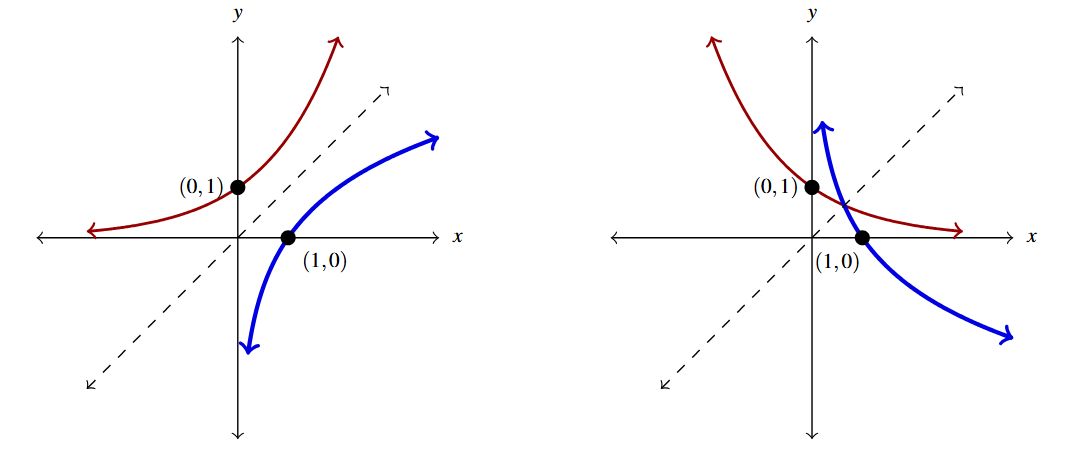
Moreover, we know the basic shapes of [latex]y = f(x) = b^{x}[/latex] (in red) for the different cases of [latex]b[/latex], thus we can obtain the graph of [latex]y = f^{-1}(x) = \log_{b}(x)[/latex] (in blue) by reflecting the graph of [latex]f[/latex] across the line [latex]y=x[/latex]. The [latex]y[/latex]-intercept [latex](0,1)[/latex] on the graph of [latex]f[/latex] corresponds to an [latex]x[/latex]-intercept of [latex](1,0)[/latex] on the graph of [latex]f^{-1}[/latex]. The horizontal asymptotes [latex]y=0[/latex] on the graphs of the exponential functions become vertical asymptotes [latex]x=0[/latex] on the log graphs.
Procedurally, logarithmic functions undo the exponential functions. Consider the function [latex]f(x) = 2^{x}[/latex]. When we evaluate [latex]f(3) = 2^{3} = 8[/latex], the input 3 becomes the exponent on the base 2 to produce the real number 8. The function [latex]f^{-1}(x) = \log_{2}(x)[/latex] then takes the number 8 as its input and returns the exponent 3 as its output. In symbols, [latex]\log_{2}(8) = 3[/latex].
More generally, [latex]\log_{2}(x)[/latex] is the exponent you put on 2 to get [latex]x[/latex]. Thus, [latex]\log_{2}(16) = 4[/latex], because [latex]2^{4} = 16[/latex]. The following theorem summarizes the basic properties of logarithmic functions, all of which come from the fact that they are inverses of exponential functions.
Suppose [latex]f(x) = \log_{b}(x)[/latex], for [latex]b>0[/latex], and [latex]b \neq 1[/latex].
- The domain of [latex]f[/latex] is [latex](0, \infty)[/latex] and the range of [latex]f[/latex] is [latex](-\infty, \infty)[/latex].
- [latex](1,0)[/latex] is on the graph of [latex]f[/latex] and [latex]x=0[/latex] is a vertical asymptote of the graph of [latex]f[/latex].
- [latex]f[/latex] is one-to-one, continuous and smooth
- [latex]b^{a} = c[/latex] if and only if [latex]\log_{b}(c) = a[/latex]. That is, [latex]\log_{b}(c)[/latex] is the exponent you put on [latex]b[/latex] to obtain [latex]c[/latex].
- [latex]\log_{b} \left(b^{x}\right) = x[/latex] for all real numbers [latex]x[/latex] and [latex]b^{\log_{b}(x)} = x[/latex] for all [latex]x > 0[/latex]
- If [latex]b > 1[/latex]:
- [latex]f[/latex] is always increasing
- As [latex]x \rightarrow 0^{+}[/latex], [latex]f(x) \rightarrow -\infty[/latex]
- As [latex]x \rightarrow \infty[/latex], [latex]f(x) \rightarrow \infty[/latex]
- The graph of [latex]f[/latex] resembles:
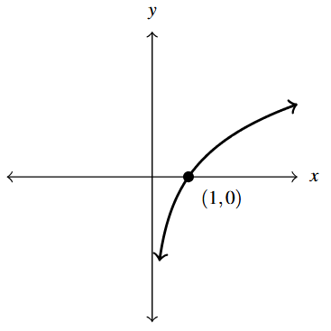
Graph of General Exponential Function for [latex] y = \log_{b} (x), \; b > 1 [/latex]
- If 0 < [latex]b[/latex] < 1:
- [latex]f[/latex] is always decreasing
- As [latex]x \rightarrow 0^{+}[/latex], [latex]f(x) \rightarrow \infty[/latex]
- As [latex]x \rightarrow \infty[/latex], [latex]f(x) \rightarrow -\infty[/latex]
- The graph of [latex]f[/latex] resembles:
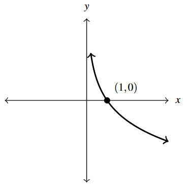
Graph of General Exponential Function for [latex] y = \log_{b} (x), \;[/latex] 0 < [latex]b [/latex] < 1
As we have mentioned, Theorem 5.5 is a consequence of Theorems 5.1 and 5.3. However, it is worth the reader’s time to understand Theorem 5.5 from an exponent perspective.
As an example, we know that the domain of [latex]g(x) = \log_{2}(x)[/latex] is [latex](0,\infty)[/latex]. Why? Because the range of [latex]f(x) = 2^{x}[/latex] is [latex](0,\infty)[/latex]. In a way, this says everything, but at the same time, it doesn’t.
To really understand why the domain of [latex]g(x) = \log_{2}(x)[/latex] is [latex](0,\infty)[/latex], consider trying to compute [latex]\log_{2}(-1)[/latex]. We are searching for the exponent we put on 2 to give us [latex]-1[/latex]. In other words, we are looking for [latex]x[/latex] that satisfies [latex]2^{x} = -1[/latex]. There is no such real number, because all powers of 2 are positive.
While what we have said is exactly the same thing as saying the domain of [latex]g(x) = \log_{2}(x)[/latex] is [latex](0,\infty)[/latex] because the range of [latex]f(x) = 2^{x}[/latex] is [latex](0,\infty)[/latex], we feel it is in a student’s best interest to understand the statements in Theorem 5.5 at this level instead of just merely memorizing the facts.
Our first example gives us practice computing logarithms as well as constructing basic graphs.
Example 5.3.1
Example 5.3.1.1a
Simplify the following: [latex]\log_{3}(81)[/latex]
Solution:
Simplify [latex]\log_{3}(81)[/latex].
The number [latex]\log_{3}(81)[/latex] is the exponent we put on 3 to get 81. As such, we want to write 81 as a power of 3.
We find [latex]81 = 3^{4}[/latex], so that [latex]\log_{3}(81)=4[/latex].
Example 5.3.1.1b
Simplify the following: [latex]\log_{2}\left(\dfrac{1}{8}\right)[/latex]
Solution:
Simplify [latex]\log_{2}\left(\dfrac{1}{8}\right)[/latex].
To find [latex]\log_{2}\left(\dfrac{1}{8}\right)[/latex], we need rewrite [latex]\dfrac{1}{8}[/latex] as a power of 2.
We find [latex]\dfrac{1}{8} = \dfrac{1}{2^{3}} = 2^{-3}[/latex], so [latex]\log_{2}\left(\dfrac{1}{8}\right) = -3[/latex].
Example 5.3.1.1c
Simplify the following: [latex]\log_{\sqrt{5}}(25)[/latex]
Solution:
Simplify [latex]\log_{\sqrt{5}}(25)[/latex].
To determine [latex]\log_{\sqrt{5}}(25)[/latex], we need to express 25 as a power of [latex]\sqrt{5}[/latex].
We know [latex]25 = 5^2[/latex], and [latex]5 = \left(\sqrt{5}\right)^2[/latex], so we have [latex]25 = \left(\left(\sqrt{5}\right)^2\right)^2 = \left(\sqrt{5}\right)^4[/latex].
We get [latex]\log_{\sqrt{5}}(25) = 4[/latex].
Example 5.3.1.1d
Simplify the following: [latex]\ln\left(\sqrt[3]{e^2}\right)[/latex]
Solution:
Simplify [latex]\ln\left(\sqrt[3]{e^2}\right)[/latex].
First, recall that the notation [latex]\ln\left(\sqrt[3]{e^2}\right)[/latex] means [latex]\log_{e}\left(\sqrt[3]{e^2}\right)[/latex], so we are looking for the exponent to put on [latex]e[/latex] to obtain [latex]\sqrt[3]{e^2}[/latex].
Rewriting [latex]\sqrt[3]{e^2} = e^{2/3}[/latex], we find [latex]\ln\left(\sqrt[3]{e^2}\right) = \ln\left(e^{2/3}\right) = \dfrac{2}{3}[/latex].
Example 5.3.1.1e
Simplify the following: [latex]\log(0.001)[/latex]
Solution:
Simplify [latex]\log(0.001)[/latex].
Rewriting [latex]\log(0.001)[/latex] as [latex]\log_{10} (0.001)[/latex], we see that we need to write 0.001 as a power of 10.
We have [latex]0.001 = \dfrac{1}{1000} = \dfrac{1}{10^3} = 10^{-3}[/latex].
Hence, [latex]\log(0.001) = \log\left(10^{-3}\right) = -3[/latex].
Example 5.3.1.1f
Simplify the following: [latex]2^{\log_{2}(8)}[/latex]
Solution:
Simplify [latex]2^{\log_{2}(8)}[/latex].
We can use Theorem 5.5 directly to simplify [latex]2^{\log_{2}(8)} = 8[/latex].
We can also understand this problem by first finding [latex]\log_{2}(8)[/latex]. By definition, [latex]\log_{2}(8)[/latex] is the exponent we put on 2 to get 2. Because [latex]8 = 2^3[/latex], we have [latex]\log_{2}(8) = 3[/latex].
We now substitute to find [latex]2^{\log_{2}(8)} = 2^3 = 8[/latex].
Example 5.3.1.1g
Simplify the following: [latex]117^{-\log_{117}(6)}[/latex]
Solution:
Simplify [latex]117^{-\log_{117}(6)}[/latex].
From Theorem 5.5, we know [latex]117^{\log_{117}(6)}=6[/latex],[1] but we cannot directly apply this formula to the expression [latex]117^{-\log_{117}(6)}[/latex] without first using a property of exponents. (Can you see why?)
Rather, we find: [latex]117^{-\log_{117}(6)} = \dfrac{1}{117^{\log_{117}(6)}} = \dfrac{1}{6}[/latex].
Example 5.3.1.2a
Graph the following functions by starting with a basic logarithmic function and using transformations, Theorem 1.12. Track at least three points and the vertical asymptote through the transformations.
[latex]F(x) = \log_{\frac{1}{3}} \left( \dfrac{x}{2} \right) + 1[/latex]
Solution:
Graph [latex]F(x) = \log_{\frac{1}{3}} \left( \dfrac{x}{2} \right) + 1.[/latex]
To graph [latex]F(x) = \log_{\frac{1}{3}} \left( \dfrac{x}{2} \right) + 1[/latex] we start with the graph of [latex]f(x) = \log_{\frac{1}{3}}(x)[/latex]. and use Theorem 1.12.
First we choose some control points on the graph of [latex]f(x) = \log_{\frac{1}{3}}(x)[/latex]. We are instructed to track three points (and the vertical asymptote, therefore [latex]x = 0[/latex]) through the transformations, we choose the points corresponding to powers of [latex]\dfrac{1}{3}[/latex]: [latex]\left( \dfrac{1}{3}, 1 \right)[/latex], [latex](1,0)[/latex], and [latex](3, -1)[/latex], respectively.
Next, we note [latex]F(x) = \log_{\frac{1}{3}} \left( \dfrac{x}{2} \right) + 1 = f \left(\dfrac{x}{2}\right) + 1[/latex]. Per Theorem 1.12, we first multiply the [latex]x[/latex]-coordinates of the points on the graph of [latex]y = f(x)[/latex] by 2, horizontally expanding the graph by a factor of 2. Next, we add 1 to the [latex]y[/latex]-coordinates of each point on this new graph, vertically shifting the graph up 1.
The horizontal asymptote, [latex]x = 0[/latex] remains unchanged under the horizontal stretch and the vertical shift.
Below we graph [latex]y = f(x) = \log_{\frac{1}{3}}(x)[/latex] on the left and [latex]y = F(x) = \log_{\frac{1}{3}} \left( \dfrac{x}{2} \right) + 1[/latex] on the right.
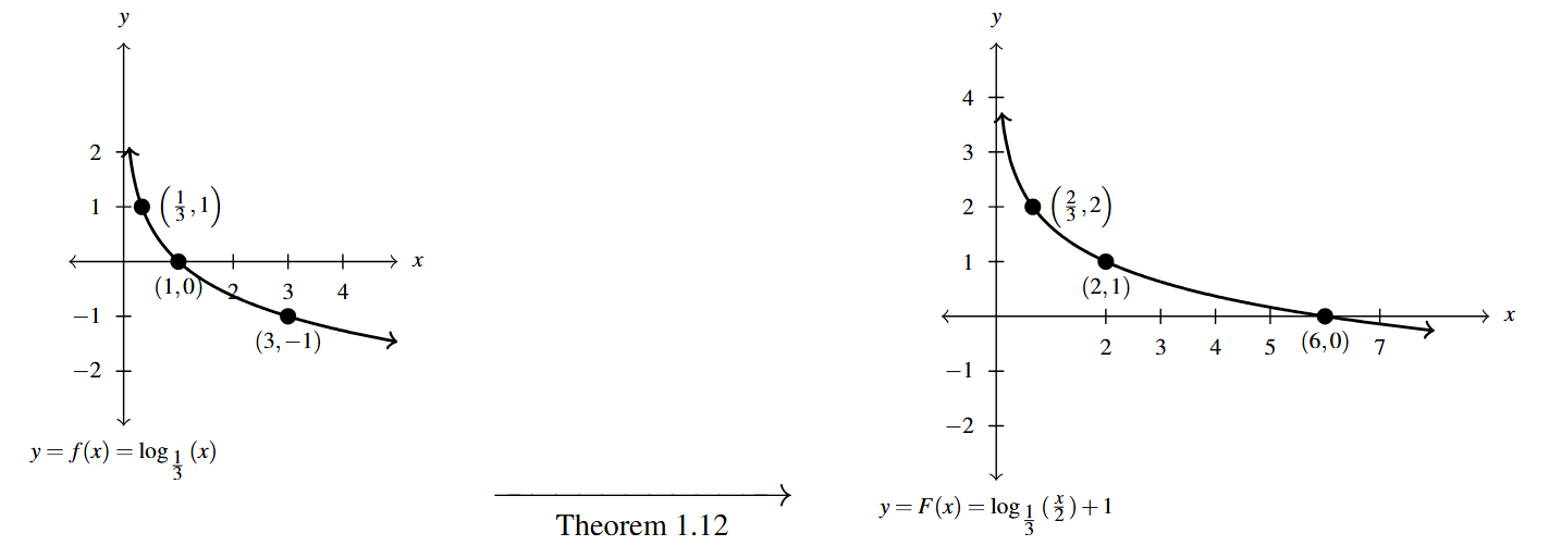
As always we can check our answer by verifying each of the points [latex]\left(\dfrac{2}{3}, 2\right)[/latex], [latex](2,1)[/latex] and [latex](6,0)[/latex], is on the graph of [latex]F(x) = \log_{\frac{1}{3}} \left( \dfrac{x}{2} \right) + 1[/latex] by checking [latex]F\left( \dfrac{2}{3} \right) = 2[/latex], [latex]F(2) = 1[/latex], and [latex]F(6) = 0[/latex]. We can check the end behavior as well, that is, as [latex]x \rightarrow 0^{+}[/latex], [latex]F(x) \rightarrow \infty[/latex] and as [latex]x \rightarrow \infty[/latex], [latex]F(x) \rightarrow -\infty[/latex]. We leave these calculations to the reader.
Example 5.3.1.2b
Graph the following functions by starting with a basic logarithmic function and using transformations, Theorem 1.12. Track at least three points and the vertical asymptote through the transformations.
[latex]G(t) =-\ln(2-t)[/latex]
Solution:
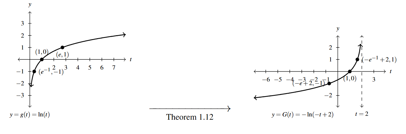
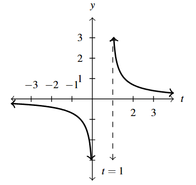
Graph [latex]G(t) =-\ln(2-t)[/latex].
Due to the fact that the base of [latex]G(t) =-\ln(2-t)[/latex] is [latex]e[/latex], we start with the graph of [latex]g(t) = \ln(t)[/latex]. [latex]e[/latex] is an irrational number, so we use the approximation [latex]e \approx 2.718[/latex] when plotting points, but label points using exact coordinates in terms of [latex]e[/latex].
We choose points corresponding to powers of [latex]e[/latex] on the graph of [latex]g(t) = \ln(t)[/latex]: [latex](e^{-1}, -1) \approx (0.368, -1)[/latex], [latex](1,0)[/latex], and [latex](e,1) \approx (2.718,1)[/latex], respectively.
[latex]G(t) =-\ln(2-t) = -\ln(-t+2) = -g(-t+2)[/latex], so Theorem 1.12 instructs us to first subtract 2 from each of the [latex]t[/latex]-coordinates of the points on the graph of [latex]g(t) = \ln(t)[/latex], shifting the graph to the left two units.
Next, we multiply (divide) the [latex]t[/latex]-coordinates of points on this new graph by [latex]-1[/latex] which reflects the graph across the [latex]y[/latex]-axis. Lastly, we multiply each of the [latex]y[/latex]-coordinates of this second graph by [latex]-1[/latex], reflecting it across the [latex]t[/latex]-axis.
Tracking points, we have [latex](e^{-1}, -1) \rightarrow (e^{-1}-2, -1) \rightarrow (-e^{-1}+2, -1) \rightarrow (- e^{-1}+2, 1) \approx ( 1.632, 1)[/latex], [latex](1,0) \rightarrow (-1,0) \rightarrow (1,0) \rightarrow (1,0)[/latex], and [latex](e,1) \rightarrow (e-2, 1) \rightarrow (-e+2,1) \rightarrow (-e+2, -1) \approx ( -0.718,-1)[/latex].
The vertical asymptote is affected by the horizontal shift and the reflection about the [latex]y[/latex]-axis only: [latex]t = 0 \rightarrow t = -2 \rightarrow t=2[/latex].
We graph [latex]g(t) = \ln(t)[/latex] below on the left and the transformed function [latex]G(t) = -\ln(-t+2)[/latex] below on the right. As usual, we can check our answer by verifying the indicated points do, in fact, lie on the graph of [latex]y = G(t)[/latex] along with checking the behavior as [latex]t \rightarrow -\infty[/latex] and [latex]t \rightarrow 2^{-}[/latex].
Example 5.3.1.3
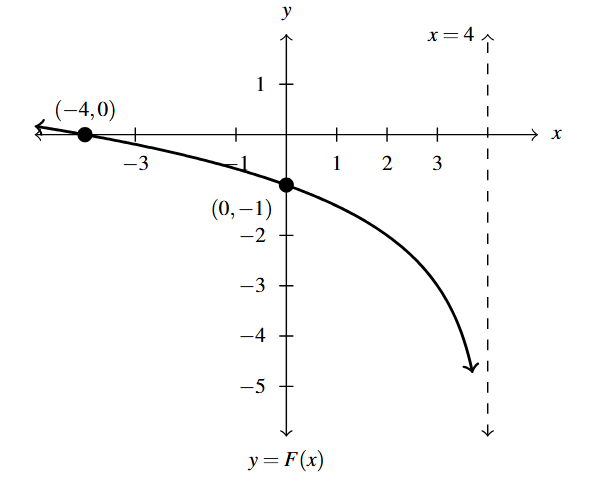
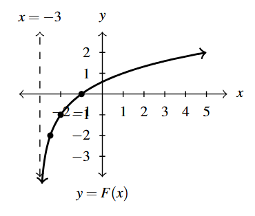
Write a formula for the graph of the function below. Assume the base of the logarithm is 2.
Solution:
Write a formula for [latex]y=F(x)[/latex], assume the base of the logarithm is 2.
We are told to assume the base of the exponential function is 2. We assume then the function [latex]F(x)[/latex] is the result of the transforming the graph of [latex]f(x) = \log_{2}(x)[/latex] using Theorem 1.12. This means we are tasked with finding values for [latex]a[/latex], [latex]b[/latex], [latex]h[/latex], and [latex]k[/latex] so that [latex]F(x) = af(bx-h)+k = a \log_{2}(bx-h)+k[/latex].
Because the vertical asymptote to the graph of [latex]y=f(x) = \log_{2}(x)[/latex] is [latex]x=0[/latex] and the vertical asymptote to the graph [latex]y = F(x)[/latex] is [latex]x=4[/latex], we know we have a horizontal shift of 4 units. Moreover, the curve approaches the vertical asymptote from the left, so we also know we have a reflection about the [latex]y[/latex]-axis and [latex]b[/latex] < 0 (this is not your base, but instead the coefficient of [latex]x[/latex].) The recipe in Theorem 1.12 instructs us to perform the horizontal shift before the reflection across the [latex]y[/latex]-axis, so we take [latex]h=-4[/latex] and assume for simplicity [latex]b = -1[/latex] so [latex]F(x) = a \log_{2}(-x+4)+k[/latex].
To determine [latex]a[/latex] and [latex]k[/latex], we make use of the two points on the graph. [latex](-4,0)[/latex] is on the graph of [latex]F[/latex], so [latex]F(-4) = a \log_{2}(-(-4)+4) + k = 0[/latex]. This reduces to [latex]a \log_{2}(8)+k = 0[/latex] or [latex]3a+k=0[/latex]. Next, we use the point [latex](0,-1)[/latex] to get [latex]F(0) = a \log_{2}(-(0)+4) +k = -1[/latex]. This reduces to [latex]a \log_{2}(4) + k = -1[/latex] or [latex]2a+k = -1[/latex]. From [latex]3a+k=0[/latex], we get [latex]k=-3a[/latex] which when substituted into [latex]2a+k=-1[/latex] gives [latex]2a +(-3a) = -1[/latex] or [latex]a = 1[/latex]. Hence, [latex]k = -3a = -3(1) = -3[/latex].
Putting all of this work together we determine [latex]F(x) = \log_{2}(-x+4)-3[/latex].
As always, we can check our answer by verifying [latex]F(-4) = 0[/latex], [latex]F(0) = -1[/latex], [latex]F(x) \rightarrow \infty[/latex] as [latex]x \rightarrow -\infty[/latex] and [latex]F(x) \rightarrow -\infty[/latex] as [latex]x \rightarrow 4^{-}[/latex]. We leave these details to the reader.[2]
Up until this point, restrictions on the domains of functions came from avoiding division by zero and keeping negative numbers from beneath even indexed radicals. With the introduction of logarithms, we now have another restriction. The argument of the logarithm[3] must be strictly positive, because the domain of [latex]f(x) = \log_{b}(x)[/latex] is [latex](0, \infty)[/latex].
Example 5.3.2
Example 5.3.2.1
State the domain each function analytically and check your answer using a graph.
[latex]f(x) = 2\log(3-x)-1[/latex]
Solution:
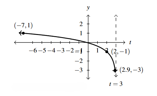
State the domain of [latex]f(x) = 2\log(3-x)-1[/latex].
We set [latex]3-x > 0[/latex] to obtain [latex]x[/latex] < 3, or [latex](-\infty, 3)[/latex].
To verify our domain, we graph [latex]f[/latex] using transformations. Taking a cue from Theorem 1.12, we rewrite [latex]f(x) = 2 \log_{10}(-x+3) -1[/latex] and view this function as a transformed version of [latex]h(x) = \log_{10}(x)[/latex].
To graph [latex]y = \log(x) = \log_{10}(x)[/latex], We select three points to track corresponding to powers of 10: [latex](0.1, -1)[/latex], [latex](1,0)[/latex] and [latex](10,1)[/latex], along with the vertical asymptote [latex]x=0[/latex].
As [latex]f(x) = 2h(-x+3)-1[/latex], Theorem 1.12 tells us that to obtain the destinations of these points, we first subtract 3 from the [latex]x[/latex]-coordinates (shifting the graph left 3 units), then divide (multiply) by the [latex]x[/latex]-coordinates by [latex]-1[/latex] (causing a reflection across the [latex]y[/latex]-axis).
Next, we multiply the [latex]y[/latex]-coordinates by 2 which results in a vertical stretch by a factor of 2, then we finish by subtracting 1 from the [latex]y[/latex]-coordinates which shifts the graph down 1 unit.
Tracking points, we find: [latex](0.1, -1) \rightarrow (-2.9, -1) \rightarrow (2.9, -1) \rightarrow (2.9, -2) \rightarrow (2.9, -3)[/latex], [latex](1,0) \rightarrow (-2,0) \rightarrow (2,0) \rightarrow (2,0) \rightarrow (2,-1)[/latex], and [latex](10,1) \rightarrow (7,1) \rightarrow (-7,1) \rightarrow (-7,2) \rightarrow (-7,1)[/latex].
The vertical shift and reflection about the [latex]y[/latex]-axis affects the vertical asymptote: [latex]x = 0 \rightarrow x = -3 \rightarrow x = 3.[/latex]
Plotting these three points along with the vertical asymptote produces the graph of [latex]f[/latex].
Example 5.3.2.2
State the domain each function analytically and check your answer using a graph.
[latex]g(x) = \ln \left(\dfrac{x}{x-1}\right)[/latex]
Solution:
State the domain of [latex]g(x) = \ln \left(\dfrac{x}{x-1}\right)[/latex].
To find the domain of [latex]g[/latex], we need to solve the inequality [latex]\dfrac{x}{x-1} > 0[/latex] using a sign diagram.[4]
If we define [latex]r(x) = \dfrac{x}{x-1}[/latex], we find [latex]r[/latex] is undefined at [latex]x=1[/latex] and [latex]r(x) = 0[/latex] when [latex]x=0[/latex]. Choosing some test values, we generate the sign diagram below.
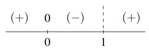
We find [latex]\dfrac{x}{x-1} > 0[/latex] on [latex](-\infty, 0) \cup (1, \infty)[/latex] which is the domain of [latex]g[/latex]. The graph below confirms this.
We can tell from the graph of [latex]g[/latex] that it is not the result of Section 1.6 transformations being applied to the graph [latex]y = \ln(x)[/latex], (do you see why?) so barring a more detailed analysis using Calculus, producing a graph using a graphing utility is the best we could do, for now.
One thing worthy of note, however, is the end behavior of [latex]g[/latex]. The graph suggests that as [latex]x \rightarrow \pm \infty[/latex], [latex]g(x) \rightarrow 0[/latex]. We can verify this analytically. Using results from Chapter 3 and continuity, we know that as [latex]x \rightarrow \pm \infty[/latex], [latex]\dfrac{x}{x-1} \approx 1[/latex]. Hence, it makes sense that [latex]g(x) = \ln \left(\dfrac{x}{x-1}\right) \approx \ln(1) = 0[/latex].
While logarithms have some interesting applications of their own which you’ll explore in the exercises, their primary use to us will be to undo exponential functions. (This is, after all, how they were defined.) Our last example reviews not only the major topics of this section, but reviews the salient points from Section 5.1.
Example 5.3.3
Example 5.3.3.1
Let [latex]f(x) = 2^{x-1} - 3[/latex].
Graph [latex]f[/latex] using transformations and state the domain and range of [latex]f[/latex].
Solution:
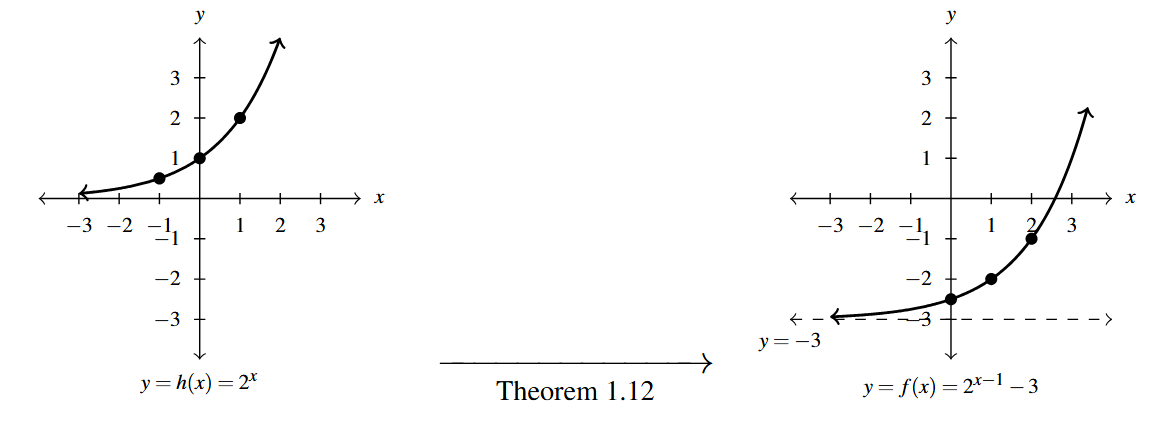
Graph [latex]f[/latex] using transformations and state the domain and range of [latex]f[/latex].
To graph [latex]f(x) = 2^{x-1} - 3[/latex] using Theorem 1.12, we first identify [latex]g(x) = 2^{x}[/latex] and note [latex]f(x) = g(x-1)-3[/latex]. Choosing the control points of [latex]\left(-1, \dfrac{1}{2}\right)[/latex], [latex](0,1)[/latex] and [latex](1, 2)[/latex] on the graph of [latex]g[/latex] along with the horizontal asymptote [latex]y=0[/latex], we implement the algorithm set forth in Theorem 1.12.
First, we first add 1 to the [latex]x[/latex]-coordinates of the points on the graph of [latex]g[/latex] which shifts the the graph of [latex]g[/latex] to the right one unit. Next, we subtract 3 from each of the [latex]y[/latex]-coordinates on this new graph, shifting the graph down 3 units to get the graph of [latex]f[/latex].
Looking point-by-point, we have [latex]\left(-1, \dfrac{1}{2}\right) \rightarrow \left(0, \dfrac{1}{2}\right) \rightarrow \left(0, -\dfrac{5}{2}\right)[/latex], [latex](0,1) \rightarrow (1,1) \rightarrow (1,-2)[/latex], and, finally, [latex](1, 2) \rightarrow (2, 2) \rightarrow (2, -1)[/latex].
The horizontal asymptote is affected only by the vertical shift, [latex]y = 0 \rightarrow y = -3[/latex].
From the graph of [latex]f[/latex], we get the domain is [latex](-\infty, \infty)[/latex] and the range is [latex](-3, \infty)[/latex].
Example 5.3.3.2
Let [latex]f(x) = 2^{x-1} - 3[/latex].
Explain why [latex]f[/latex] is invertible and find a formula for [latex]f^{-1}(x)[/latex].
Solution:
Explain why [latex]f[/latex] is invertible and find a formula for [latex]f^{-1}(x)[/latex].
The graph of [latex]f[/latex] passes the Horizontal Line Test so [latex]f[/latex] is one-to-one, hence invertible.
To find a formula for [latex]f^{-1}(x)[/latex], we normally set [latex]y=f(x)[/latex], interchange the [latex]x[/latex] and [latex]y[/latex], then proceed to solve for [latex]y[/latex]. Doing so in this situation leads us to the equation [latex]x = 2^{y-1}-3[/latex]. We have yet to discuss how to solve this kind of equation, so we will attempt to find the formula for [latex]f^{-1}[/latex] procedurally.
Thinking of [latex]f[/latex] as a process, the formula [latex]f(x) = 2^{x-1}-3[/latex] takes an input [latex]x[/latex] and applies the steps: first subtract 1. Second put the result of the first step as the exponent on 2. Last, subtract 3 from the result of the second step.
Clearly, to undo subtracting 1, we will add 1, and similarly we undo subtracting 3 by adding 3. How do we undo the second step? The answer is we use the logarithm.
By definition, [latex]\log_{2}(x)[/latex] undoes exponentiation by 2. Hence, [latex]f^{-1}[/latex] should: first, add 3. Second, take the logarithm base 2 of the result of the first step. Lastly, add 1 to the result of the second step. In symbols, [latex]f^{-1}(x) = \log_{2}(x+3)+1[/latex].
Example 5.3.3.3
Let [latex]f(x) = 2^{x-1} - 3[/latex].
Graph [latex]f^{-1}[/latex] using transformations and state the domain and range of [latex]f^{-1}[/latex].
Solution:
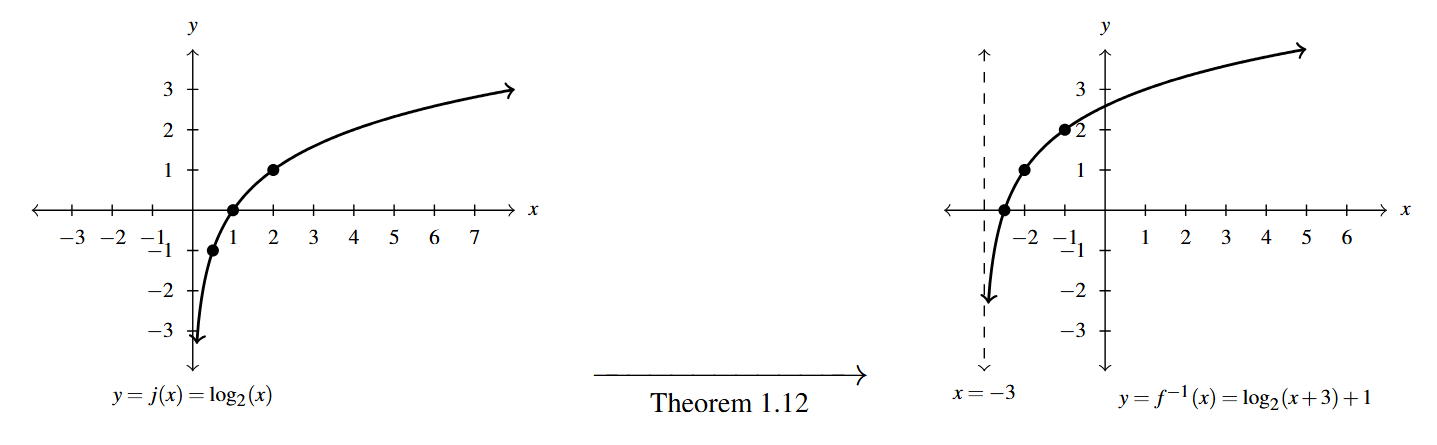
Graph [latex]f^{-1}[/latex] using transformations and state the domain and range of [latex]f^{-1}[/latex].
To graph [latex]f^{-1}(x) = \log_{2}(x+3)+1[/latex] using Theorem 1.12, we start with [latex]j(x) = \log_{2}(x)[/latex] and track the points [latex]\left(\dfrac{1}{2},-1\right)[/latex], [latex](1,0)[/latex] and [latex](2, 1)[/latex] on the graph of [latex]j[/latex] along with the vertical asymptote [latex]x=0[/latex] through the transformations.
As [latex]f^{-1}(x) = j(x+3)+1[/latex], we first subtract 3 from each of the [latex]x[/latex]-coordinates of each of the points on the graph of [latex]y=j(x)[/latex] shifting the graph of [latex]j[/latex] to the left three units. We then add 1 to each of the [latex]y[/latex]-coordinates of the points on this new graph, shifting the graph up one unit.
Tracking points, we get [latex]\left(\dfrac{1}{2},-1\right) \rightarrow \left(-\dfrac{5}{2},-1\right) \rightarrow \left(-\dfrac{5}{2},0\right)[/latex], [latex](1,0) \rightarrow (-2,1) \rightarrow (-2,2)[/latex], and [latex](2, 1) \rightarrow (-1, 1) \rightarrow (-1, 2)[/latex].
The vertical asymptote is only affected by the horizontal shift, so we have [latex]x = 0 \rightarrow x = -3[/latex].
From the graph below, we get the domain of [latex]f^{-1}[/latex] is [latex](-3, \infty)[/latex], which matches the range of [latex]f[/latex], and the range of [latex]f^{-1}[/latex] is [latex](-\infty, \infty)[/latex], which matches the domain of [latex]f[/latex], in accordance with Theorem 5.1.
Example 5.3.3.4
Let [latex]f(x) = 2^{x-1} - 3[/latex].
Verify [latex]\left(f^{-1} \circ f\right)(x) = x[/latex] for all [latex]x[/latex] in the domain of [latex]f[/latex] and [latex]\left(f \circ f^{-1} \right)(x) = x[/latex] for all [latex]x[/latex] in the domain of [latex]f^{-1}[/latex].
Solution:
Verify [latex]\left(f^{-1} \circ f\right)(x) = x[/latex] for all [latex]x[/latex] in the domain of [latex]f[/latex] and [latex]\left(f \circ f^{-1} \right)(x) = x[/latex] for all [latex]x[/latex] in the domain of [latex]f^{-1}[/latex].
We now verify that [latex]f(x) = 2^{x-1}-3[/latex] and [latex]f^{-1}(x) = \log_{2}(x+3)+1[/latex] satisfy the composition requirement for inverses. When simplifying [latex](f^{-1} \circ f)(x)[/latex] we assume [latex]x[/latex] can be any real number while when simplifying [latex](f \circ f^{-1})(x)[/latex], we restrict our attention to [latex]x > -3[/latex]. (Do you see why?)
Note the use of the inverse properties of exponential and logarithmic functions from Theorem 5.5 when it comes to simplifying expressions of the form [latex]\log_{2}(2^{u})[/latex] and [latex]2^{\log_{2}(u)}[/latex].
\[ \begin{array}{ccc} \begin{array}{rcl}
\left(f^{-1}\circ f\right)(x) & = & f^{-1}(f(x)) \\
& = & f^{-1}\left(2^{x-1}-3 \right) \\
& = & \log_{2}\left( \left[2^{x-1}-3\right]+3 \right)+1 \\
& = & \log_{2}\left( 2^{x-1} \right)+1 \\
& = & (x-1) +1 \\
& = & x \, \, \checkmark \\ \end{array} & \quad & \begin{array}{rcl}
\left(f\circ f^{-1}\right)(x) & = & f\left(f^{-1}(x)\right) \\
& = & f\left( \log_{2}(x+3)+1 \right) \\
& = & 2^{\left( \log_{2}(x+3)+1 \right)-1} – 3 \\
& = & 2^{\log_{2}(x+3)} – 3 \\
& = & (x+3) -3 \\
& = & x \, \, \checkmark \\ \end{array} \end{array} \]
Example 5.3.3.5
Let [latex]f(x) = 2^{x-1} - 3[/latex].
Graph [latex]f[/latex] and [latex]f^{-1}[/latex] on the same set of axes and check for symmetry about the line [latex]y = x[/latex].
Solution:
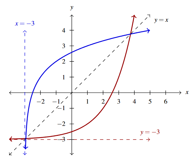
Graph [latex]f[/latex] and [latex]f^{-1}[/latex] on the same set of axes and check for symmetry about the line [latex]y = x[/latex].
Last, but certainly not least, we graph [latex]y=f(x)[/latex] (in red) and [latex]y=f^{-1}(x)[/latex] (in blue) on the same set of axes and observe the symmetry about the line [latex]y=x[/latex].
Example 5.3.3.6a
Let [latex]f(x) = 2^{x-1} - 3[/latex].
Use [latex]f[/latex] or [latex]f^{-1}[/latex] to solve the following equations. Check your answers algebraically.
[latex]2^{x-1} - 3 = 4[/latex]
Solution:
Use [latex]f[/latex] or [latex]f^{-1}[/latex] to solve [latex]2^{x-1} - 3 = 4.[/latex]
Viewing [latex]2^{x-1} - 3 = 4[/latex] as [latex]f(x) = 4[/latex], we apply [latex]f^{-1}[/latex] to undo [latex]f[/latex] to get [latex]f^{-1}(f(x)) = f^{-1}(4)[/latex], which reduces to [latex]x = f^{-1}(4)[/latex]. We have shown (algebraically and graphically!) that [latex]f^{-1}(x) = \log_{2}(x+3) + 1[/latex], we get [latex]x = f^{-1}(4) = \log_{2}(4+3) + 1 = \log_{2}(7) + 1.[/latex]
Alternatively, we know from Theorem 5.1 that [latex]f(x) = 4[/latex] is equivalent to [latex]x = f^{-1}(4)[/latex] directly.
Note that, by definition, [latex]2^{\log_{2}(7)} = 7[/latex], thus [latex]2^{( \log_{2}(7) + 1)-1} - 3 = 2^{\log_{2}(7)} - 3 = 7 - 3 = 4[/latex], as required.
Example 5.3.3.6b
Let [latex]f(x) = 2^{x-1} - 3[/latex].
Use [latex]f[/latex] or [latex]f^{-1}[/latex] to solve the following equations. Check your answers algebraically.
[latex]\log_{2}(t+3)+1 = 0[/latex]
Solution:
Use [latex]f[/latex] or [latex]f^{-1}[/latex] to solve [latex]\log_{2}(t+3)+1 = 0.[/latex]
Because we may think of the equation [latex]\log_{2}(t+3)+1 = 0[/latex] as [latex]f^{-1}(t) = 0[/latex], we can solve this equation by applying [latex]f[/latex] to both sides to get [latex]f(f^{-1}(t)) = f(0)[/latex] or [latex]t = 2^{0-1} -3 = \dfrac{1}{2} - 3 = -\dfrac{5}{2}.[/latex]
As a result of [latex]\log_{2}(2^{-1}) = -1[/latex], we get [latex]\log_{2}\left(-\dfrac{5}{2} +3 \right)+1 = \log_{2}\left( \dfrac{1}{2} \right) + 1 = \log_{2}(2^{-1})-1 + 1 = 0[/latex], as required.
5.3.1 Section Exercises
In Exercises 1 – 15, use the property: [latex]b^{a} = c[/latex] if and only if [latex]\log_{b}(c) = a[/latex] from Theorem 5.5 to rewrite the given equation in the other form. That is, rewrite the exponential equations as logarithmic equations and rewrite the logarithmic equations as exponential equations.
- [latex]2^{3} = 8[/latex]
- [latex]5^{-3} = \dfrac{1}{125}[/latex]
- [latex]4^{5/2} = 32[/latex]
- [latex]\left(\dfrac{1}{3}\right)^{-2} = 9[/latex]
- [latex]\left(\dfrac{4}{25}\right)^{-1/2} = \dfrac{5}{2}[/latex]
- [latex]10^{-3} = 0.001[/latex]
- [latex]e^{0} = 1[/latex]
- [latex]\log_{5}(25) = 2[/latex]
- [latex]\log_{25} (5) = \dfrac{1}{2}[/latex]
- [latex]\log_{3} \left(\dfrac{1}{81} \right) = -4[/latex]
- [latex]\log_{\frac{4}{3}} \left(\dfrac{3}{4} \right) = -1[/latex]
- [latex]\log(100) = 2[/latex]
- [latex]\log (0.1) = -1[/latex]
- [latex]\ln(e) = 1[/latex]
- [latex]\ln\left(\dfrac{1}{\sqrt{e}}\right) = -\dfrac{1}{2}[/latex]
In Exercises 16 – 42, evaluate the expression without using a calculator.
- [latex]\log_{3} (27)[/latex]
- [latex]\log_{6} (216)[/latex]
- [latex]\log_{2} (32)[/latex]
- [latex]\log_{6} \left( \dfrac{1}{36} \right)[/latex]
- [latex]\log_{8} (4)[/latex]
- [latex]\log_{36} (216)[/latex]
- [latex]\log_{\frac{1}{5}} (625)[/latex]
- [latex]\log_{\frac{1}{6}} (216)[/latex]
- [latex]\log_{36} (36)[/latex]
- [latex]\log \left(\dfrac{1}{1000000}\right)[/latex]
- [latex]\log(0.01)[/latex]
- [latex]\ln\left(e^3\right)[/latex]
- [latex]\log_{4} (8)[/latex]
- [latex]\log_{6} (1)[/latex]
- [latex]\log_{13} \left(\sqrt{13}\right)[/latex]
- [latex]\log_{36} \left(\sqrt[4]{36}\right)[/latex]
- [latex]7^{\log_{7} (3)}[/latex]
- [latex]36^{\log_{36}(216)}[/latex]
- [latex]\log_{36} \left(36^{216}\right)[/latex]
- [latex]\ln \left(e^{5} \right)[/latex]
- [latex]\log \left(\sqrt[9]{10^{11}}\right)[/latex]
- [latex]\log\left( \sqrt[3]{10^5} \right)[/latex]
- [latex]\ln \left( \dfrac{1}{\sqrt{e}}\right)[/latex]
- [latex]\log_{5} \left(3^{\log_{3} (5)}\right)[/latex]
- [latex]\log\left(e^{\ln(100)}\right)[/latex]
- [latex]\log_{2}\left(3^{-\log_{3}(2)}\right)[/latex]
- [latex]\ln\left(42^{6\log(1)}\right)[/latex]
In Exercises 43 – 57, find the domain of the function.
- [latex]f(x) = \ln(x^{2} + 1)[/latex]
- [latex]f(x) = \log_{7}(4x + 8)[/latex]
- [latex]g(t) = \ln(4t-20)[/latex]
- [latex]g(t) = \log \left(t^2+9t+18\right)[/latex]
- [latex]f(x) = \log \left(\dfrac{x + 2}{x^{2} - 1}\right)[/latex]
- [latex]f(x) = \log\left(\dfrac{x^2+9x+18}{4x-20}\right)[/latex]
- [latex]g(t) = \ln(7 - t) + \ln(t - 4)[/latex]
- [latex]g(t) = \ln(4t-20) + \ln\left(t^2+9t+18\right)[/latex]
- [latex]f(x) = \log\left(x^2+x+1\right)[/latex]
- [latex]f(x) = \sqrt[4]{\log_{4} (x)}[/latex]
- [latex]g(t) = \log_{9}(|t + 3| - 4)[/latex]
- [latex]g(t) = \ln(\sqrt{t - 4} - 3)[/latex]
- [latex]f(x) = \dfrac{1}{3 - \log_{5} (x)}[/latex]
- [latex]f(x) = \dfrac{\sqrt{-1 - x}}{\log_{\frac{1}{2}} (x)}[/latex]
- [latex]f(x) = \ln(-2x^{3} - x^{2} + 13x - 6)[/latex]
In Exercises 58 – 65, sketch the graph of [latex]y=g(x)[/latex] by starting with the graph of [latex]y = f(x)[/latex] and using transformations. Track at least three points of your choice and the vertical asymptote through the transformations. State the domain and range of [latex]g[/latex].
- [latex]f(x) = \log_{2}(x)[/latex] and [latex]g(x) = \log_{2}(x+1)[/latex]
- [latex]f(x) = \log_{\frac{1}{3}}(x)[/latex] and [latex]g(x) = \log_{\frac{1}{3}}(x)+1[/latex]
- [latex]f(x) = \log_{3}(x)[/latex] and [latex]g(x) = -\log_{3}(x-2)[/latex]
- [latex]f(x) = \log(x)[/latex] and [latex]g(x) = 2\log(x+20) -1[/latex]
- [latex]g(t) = \log_{0.5}(t)[/latex] and [latex]g(t) = 10 \log_{0.5}\left(\dfrac{t}{100}\right)[/latex]
- [latex]g(t) = \log_{1.25}(t)[/latex] and [latex]g(t) = \log_{1.25}(-t+1) + 2[/latex]
- [latex]g(t) = \ln(t)[/latex] and [latex]g(t) = -\ln(8-t)[/latex]
- [latex]g(t) = \ln(t)[/latex] and [latex]g(t) = -10\ln\left(\dfrac{t}{10}\right)[/latex]
In Exercises 66 – 69, the graph of a logarithmic function is given. Find a formula for the function in the form [latex]F(x) = a \cdot \log_{2}(bx-h)+k[/latex].
- Points: [latex]\left( -\dfrac{5}{2}, -2 \right)[/latex], [latex]\left(-2, -1 \right)[/latex], [latex]\left(-1,0 \right)[/latex], Asymptote: [latex]x = -3[/latex]
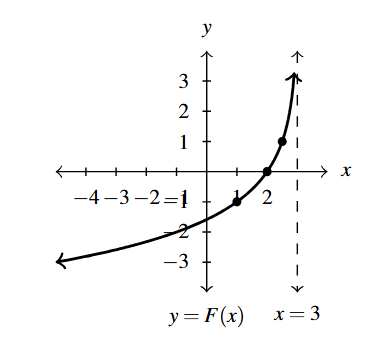
Graph for Exercise 66 - Points: [latex]\left( 1, -1 \right)[/latex], [latex]\left( 2, 0 \right)[/latex], [latex]\left(\dfrac{5}{2}, 1 \right)[/latex], Asymptote: [latex]x = 3[/latex]
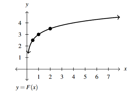
Graph for Exercise 67 - Points: [latex]\left(\dfrac{1}{2}, \dfrac{5}{2} \right)[/latex], [latex]\left(1, 3 \right)[/latex], [latex]\left(2, \dfrac{7}{2} \right)[/latex], Asymptote: [latex]x = 0[/latex]
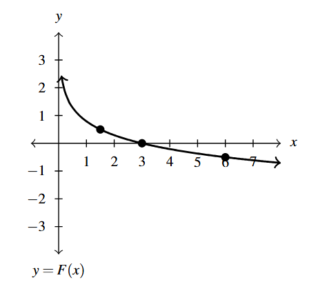
Graph for Exercise 68 - Points: [latex]\left( 6, -\dfrac{1}{2} \right)[/latex], [latex]\left(3,0 \right)[/latex], [latex]\left( \dfrac{3}{2}, \dfrac{1}{2} \right)[/latex], Asymptote: [latex]x = 0[/latex]
Graph for Exercise 69 - Find a formula for each graph in Exercises 66 – 69 of the form [latex]G(x) = a \cdot \log_{4}(bx-h)+k[/latex].
In Exercises 71 – 74, find the inverse of the function from the procedural perspective discussed in Example 5.3.3 and graph the function and its inverse on the same set of axes.
- [latex]f(x) = 3^{x + 2} - 4[/latex]
- [latex]f(x) = \log_{4}(x - 1)[/latex]
- [latex]g(t)= -2^{-t} + 1[/latex]
- [latex]g(t) = 5\log(t) - 2[/latex]
In Exercises 75 – 80, write the given function as a nontrivial decomposition of functions as directed.
- For [latex]f(x) = \log_{2}(x+3) + 4[/latex], find functions [latex]g[/latex] and [latex]h[/latex] so that [latex]f=g+h[/latex].
- For [latex]f(x) = \log(2x) - e^{-x}[/latex], find functions [latex]g[/latex] and [latex]h[/latex] so that [latex]f=g-h[/latex].
- For [latex]f(t) = 3t \log(t)[/latex], find functions [latex]g[/latex] and [latex]h[/latex] so that [latex]f=gh[/latex].
- For [latex]r(x) = \dfrac{\ln(x)}{x}[/latex], find functions [latex]f[/latex] and [latex]g[/latex] so [latex]r = \dfrac{f}{g}[/latex].
- For [latex]k(t) = \ln(t^2+1)[/latex], find functions [latex]f[/latex] and [latex]g[/latex] so that [latex]k = g \circ f[/latex].
- For [latex]p(z) = (\ln(z))^2[/latex], find functions [latex]f[/latex] and [latex]g[/latex] so [latex]p = g \circ f[/latex].
- Earthquakes are complicated events and it is not our intent to provide a complete discussion of the science involved in them. Instead, we refer the interested reader to a solid course in Geology[5] or the U.S. Geological Survey’s Earthquake Hazards Program and present only a simplified version of the Richter scale. The Richter scale measures the magnitude of an earthquake by comparing the amplitude of the seismic waves of the given earthquake to those of a “magnitude 0 event”, which was chosen to be a seismograph reading of 0.001 millimeters recorded on a seismometer 100 kilometers from the earthquake’s epicenter. Specifically, the magnitude of an earthquake is given by \[M(x) = \log \left(\dfrac{x}{0.001}\right)\] where [latex]x[/latex] is the seismograph reading in millimeters of the earthquake recorded 100 kilometers from the epicenter.
- Show that [latex]M(0.001) = 0[/latex].
- Compute [latex]M(80,000)[/latex].
- Show that an earthquake which registered 6.7 on the Richter scale had a seismograph reading ten times larger than one which measured 5.7.
- Find two news stories about recent earthquakes which give their magnitudes on the Richter scale. How many times larger was the seismograph reading of the earthquake with larger magnitude?
- While the decibel scale can be used in many disciplines,[6] we shall restrict our attention to its use in acoustics, specifically its use in measuring the intensity level of sound. The Sound Intensity Level [latex]L[/latex] (measured in decibels) of a sound intensity [latex]I[/latex] (measured in watts per square meter) is given by \[L(I) = 10\log\left( \dfrac{I}{10^{-12}} \right).\] Like the Richter scale, this scale compares [latex]I[/latex] to baseline: [latex]10^{-12} \dfrac{W}{m^{2}}[/latex] is the threshold of human hearing.
- Compute [latex]L(10^{-6})[/latex].
- Damage to your hearing can start with short term exposure to sound levels around 115 decibels. What intensity [latex]I[/latex] is needed to produce this level?
- Compute [latex]L(1)[/latex]. How does this compare with the threshold of pain which is around 140 decibels?
- The pH of a solution is a measure of its acidity or alkalinity. Specifically, [latex]\text{pH} = -\log[\text{H}^{+}][/latex] where [latex][\text{H}^{+}][/latex] is the hydrogen ion concentration in moles per liter. A solution with a pH less than 7 is an acid, one with a pH greater than 7 is a base (alkaline) and a pH of 7 is regarded as neutral.
- The hydrogen ion concentration of pure water is [latex][\text{H}^{+}] = 10^{-7}[/latex].
- Find the pH of a solution with [latex][\text{H}^{+}] = 6.3 \times 10^{-13}[/latex].
- The pH of gastric acid (the acid in your stomach) is about 0.7. What is the corresponding hydrogen ion concentration?
- Use the definition of logarithm to explain why [latex]\log_{b} 1 = 0[/latex] and [latex]\log_{b} b = 1[/latex] for every [latex]b > 0, \; b \neq 1[/latex].
Section 5.3 Exercise Answers can be found in the Appendix.
- It is worth a moment of your time to think your way through why [latex]117^{\log_{117}(6)}=6[/latex]. By definition, [latex]\log_{117}(6)[/latex] is the exponent we put on 117 to get 6. What are we doing with this exponent? We are putting it on 117, so we get 6. ↵
- As with Example 5.2.1 in Section 5.2, we may well wonder if our solution to this problem is the only solution because we made a simplifying assumption that [latex]b=-1[/latex]. We leave this for a thoughtful discussion in Exercise 40 in Section 5.4. ↵
- that is, what's inside the log ↵
- See Section 3.3 for a review of this process, if needed. ↵
- Rock-solid, perhaps? ↵
- See this webpage for the decibel scale for more information. ↵
The logarithmic function is the inverse function for the exponential function of the same base.
