Introduction to Modeling

Jeremiah Green

10 Introduction to Modeling

Learning Objectives

Explain modeling steps
Describe modeling design
Define modeling principles
Describe strengths and weaknesses of modeling techniques for decision making

Chapter content

This chapter will work to create intuition for how all models work. We will define terms, lay out principles, and provide examples. In later chapters, we will use the intuition from this chapter to provide more details. For now, when details are shown here, work to develop the modeling intuition rather than the specific details by which the modeling occurs.

Modeling steps

This image dispays the process for modeling in three steps: 1. Find patterns in the training data, 2. assume the same patterns for new data, 3. make predictions — Modeling process

All models use training data to find patterns. Different modeling methods have different objectives and use the training data in different ways, but the goal of finding patterns that can be used to make inferences in new data is common to all modeling methods. The biggest differences between models is the type of pattern that a model seeks to identify in the training data. After a model is trained, the patterns from the training data are assumed to apply to new data. The patterns from the training data are then combined with the new data to make predictions. Statistical, econometric, and machine learning models are not deterministic. That means that the predictions are uncertain estimates based on training data patterns.

A simple example helps illustrate the modeling steps. The figure below details the modeling process with this example.

This image gives a case for the example model process. (1) observe that controls and incentives are associated with misstatements. (2) Assume that client characteristics will be correlated with misstatements. (3) Predict the probability of misstatement. — Example model process

Suppose you are an auditor and want to predict whether the inventory account is likely to be misstated. To make the prediction, you draw on your own or others’ past experience with similar clients. Based on this experience, you observe that client characteristics are correlated with mistatements. For example, you might observe that clients in the same industry with ineffective controls and strong incentives have misstated ending inventory balances while clients with effective controls and/or weak incentives have not misstated their inventory balances. Your observed correlations are your model, intuitive or otherwise, of how client characteristics are associated with misstatements. Based on this model, you assume that for a new client its characteristics and misstatements will be correlated in the same way. Specifically, you assume that clients with ineffective controls and strong incentives will be more likely to have misstated inventory than clients with effective controls and/or weak incentives. Finally, you note your client’s characteristics. Suppose that this client has effective controls and weak incentives. Based on your model and your client’s characteristics, you predict that your client is unlikely to have misstated inventory.

Modeling design

There are many different types of models. This book divides models into two categories: unsupervised and supervised models. Unsupervised models are models that are used to detect patterns in data but do not have an observed outcome. Supervised models are used to model and predict an outcome variable. More details about the types of models and specific models are discussed in the relevant chapters. This section explains general model design steps that apply to all models.

The following are generic steps for a model algorithm.

Model algorithm

1. Specify a pattern

2. Define fit

3. Find the parameters that maximize fit

Technical details for modeling design

The details for how the algorithm is applied depend on the model. Here we will walk through two examples of how the algorithm for a supervised learning model could be applied. We will first be general and then we will be more specific.

General

Specify a pattern

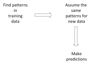
The first step is choosing a pattern that a model should identify. Patterns in the data tell us the expected associations between predictor and outcome variables. Because there may be random causes of the outcome variable, the expected associations tell us what is typical based on the variables and patterns we observe. Note that we expect to be wrong because we will not be able to perfectly model the outcome variables.

A pattern can be identified with specified data and parameters. For example, the data could be a vector that contains company age for a set of 100 companies and another column that contains number of employees for the same companies. A parameter could be the correlation between company age and number of employees. For example, this might be a correlation 70% saying that the age of the company is 70% correlated with number of employees.

A general form of this could be stated as follows, where X is a data matrix made of up x for entity i at time t, β is a set of parameters, and Y is a vector of outcomes y for entity i at time t that we want to model.

$Y = fun(\beta,X)$

This general form means that we have an observed outcome Y that we want to explain or predict. “fun” indicates that whatever pattern we do find is a function of the data X and the parameters β. The parameters β are unknown. We will use the data to estimate them.

Define fit

From this general model, we need to determine what makes the model a good fit for the data. Because the data X is already given, we only have β to work with. A measure of model fit defines for the algorithm what a good set of βs are. Define a prediction from the model as $\hat{Y}$ . This means that whatever pattern we find using the β and X, the predicted vector of outcomes is given by $\hat{Y}$ . There are different ways to define fit such as mean absolute error or r-squared. The specific way to define fit is not important here, but we will use mean absolute error (MAE) to discuss it.

$MAE= \frac{\sum_1^N |y_{i,t}-\hat{y_{i,t}}|}{N}$

This measure of fit compares the predicted value for each observation $\hat{y_{i,t}}$ with the actual outcome $y_{i,t}$ . The absolute value of the difference is a measure of how close the model prediction is to the outcome. Summarizing across all predictions and outcomes, in this case using the mean of the absolute error, captures a summary of how the model fits observations across all outcomes. Another common way to summarize the fit include summing the squared value of the errors (mean squared error). The larger the MSE, the worse the model fits the observed outcome.

Find the parameters that maximize fit

With the pattern selected and the fit defined, model estimation involves choosing the parameters that best fit the data. This might take the following form.

$\begin{equation*} \begin{aligned} & \underset{\beta}{\text{min}} & & MAE \end{aligned} \end{equation*}$

This optimization sets the objective to minimize MAE, i.e. maximize model fit, by choosing the β parameters.

Returning to the modeling steps, once the model is estimated on training data, the model, now with βs set based on the training data, the parameters are assumed to be applied to a different data set. For example, Z rather than X. In this case, the βs are combined with Z to make predictions for the new data set.

Specific

The steps above might be applied to a specific case. The patterns that determine what is typical depend on mathematical representations of how well the model fits the data. However, to find patterns in the data, we need to propose a structure that we hope might capture these patterns. There are many algorithms for measuring how well a model fits the data and many modeling structures for identifying patterns in the data. For a specific example, suppose that we propose a linear model of the data. To make the concept tractable, let’s assume that we are trying to predict a fine that a company has to pay after committing fraud. Suppose we have a few hundred observations. Below shows you a few rows of the data. Note that I am making up numbers for the purpose of the example.

Fraud fine data

Row ID	Fine Amount	Fraud Damage Amount	Prior Fraud Committed	Company Size
1	$300	$500	0	$25,000
2	$1,550	$750	1	$100,000
3	$725	$1,000	0	$15,000

Here, the outcome that we want to model and later predict is “Fine Amount”. “Fraud Damage Amount” is how much company owners lost because of the fraud. “Prior Fraud Committed” is equal to 1 if the company previously committed fraud and 0 otherwise. “Company Size” is the company’s cash account balance. Suppose we propose the following linear model.

$\bigskip$

$\begin{equation*} \begin{aligned} & y_{i,t} = & & \beta_1 Fraud Damage Amount_{i,t} +&&\beta_2 Prior Fraud Commited_{i,t} +\end{aligned} \end{equation*}$

$\begin{equation*} \begin{aligned} & \beta_3 Company Size_{i,t}&&+ \epsilon_{i,t}\end{aligned} \end{equation*}$

$\bigskip$

This equation proposes that the data, here three different columns (Fraud Damage Amount, Prior Fraud Commited, and Company Size), are combined in a linear way with $\beta_1$ , $\beta_2$ , and $\beta_3$ , to determine the fine amount. We might make this more specific with the data example above.

Linear model

Fine Amount

Fraud Damage Amount

Prior Fraud Committed

Company Size

$300

=

β₁

$500

+

β₂

0

+

β₃

$25,000

+

ε₁

$1,550

=

β₁

$750

+

β₂

1

+

β₃

$100,000

+

ε₂

$725

=

β₁

$1,000

+

β₂

0

+

β₃

$15,000

+

ε₃

Notice that each row represents an equation. We are proposing that β₁ is constant across all rows and that this parameter tells us how the “Fraud Damage Amount” is associated with “Fine Amount”. This could be thought of as the partial correlation between “Fraud Damage Amount” and “Fine Amount”. We apply the same logic to β₂ and β₃. We don’t know what these value are. These values are also not deterministic so that there is not a unique solution where the math lines up perfectly. Because we are proposing the structure and trying to find the parameters that seem to reflect what is in the data, we need the final piece of the equation which is the error term at the end. The error term is the value that makes the equation balance. Another way to think of this is that we are looking for the parameters that are typical for the data and anything that differs from what is typical is captured by the error term.

Once we have this structure, the same steps apply. We define model fit and maximize model fit by choosing the best βs.

Modeling definitions and principles

Training data

Training data includes outcomes we want to predict and data that can be used to make the predictions. For most modeling applications, we need individual observations (rows) that have data for the outcome we want to predict. In standard linear regression models, this is the “y” variable that we want to model on the training data and then predict for new data for which we do not know the outcome.We also need other information about individual observations that can be used to explain and then predict the outcome variable (the “x” variables). We collect and/or create these variables and store these as different columns. The better our columns are for predicting the outcome, the better our model will perform.

Testing data

Testing data (new data that the model will be applied to) requires “x” variables to make predictions before the outcomes are observed. The predictor columns must be available even when the outcome variable is not available and must apply to each observation.

Assumption that patterns apply to new data may be wrong

The risk from applying patterns to new data is significant and we use methods to try to reduce that risk. After using the training data to develop our models, we move to predicting outcomes. We take the same structure to new data where we do not observe the outcome to predict what we think it would be based on the model we estimate on the training data.

How well the training data model predicts outcomes on new data depends on many factors. The following outlines some of the biggest concerns.

Another concern is the interpretation of patterns in data. Correlation is a statistical property of how two (or more) variables move together. Two variables can move together because one variable causes the other. For example, dropping a ball from varying heights causes the ball to bounce higher. Two variables could also move together because a third variable causes them to move together. The third variable may be part of the causal chain relating the two variables, for example, the force the ground exerts on the ball when it hits causes the ball to bounce. In this case dropping the ball might be said to cause the ball to bounce even though it is not the proximate cause. The third variable may be not related to the causal chain and in this case the correlation between the first two variables is only driven by a spurious correlated variable. Alternatively, two variables may be correlated by chance. These correlations then are spurious and imply no form of causation.

Some practices help limit the impact of these problems in modeling. These include:

Be careful and think critically before analyzing data.
Only work with training data that is representative of the population of interest.
Keep testing separate and only use it once after all model development is complete.

Applying models to decision making

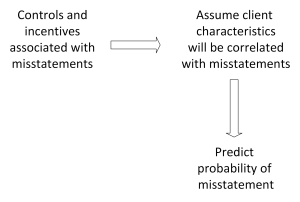
Data analysis is useful if it informs decision making. Empirical models can inform decision making in at least two ways. First, modeling may uncover patterns in data that inform how decision makers think about problems. For instance, a model might show the accounts that are most commonly associated with fraud. The model therefore informs how decision makers think about controls or detecting fraud. Second, modeling may provide useful predictions. For example, predicting which individuals most likely avoid taxes informs IRS decision makers about how to allocate time and resources.

In addition to the concerns from the previous section, whether modeling is useful for decision makers depends on many factors. Some of the strengths and weaknesses of modeling tools are listed below.

Strengths

Can include many variables that affect outcomes.
Can include interactions, non-linearities, or other complex associations.
Can synthesize information from large data sets.
Effectiveness of predictions can be tested.
Can be designed for specific questions and problems.

Weaknesses

Requires data to train a model.
A model may not be a good representation of reality.
Data may not contain outcomes or important predictors.
A good training data model may not generalize to new data.
Model may not directly address what decision makers need.

Whether modeling is an appropariate or useful tool or which modeling tool is useful depends on the circumstances. Subsequent chapters will describe and demonstrate modeling tools and some of their applications.

Conclusion

In this chapter, you learned about the model process, modeling design, and modeling principles. You also learned about the strengths and weakenesses of modeling as a data analysis tool.

Review

Mini case video

Yang Bao, Bin Ke, Bin Li, Julia Yu, and Jie Zhang (2020). Detecting Accounting Fraud in Publicly Traded U.S. Firms Using a Machine Learning Approach. Journal of Accounting Research, 58 (1): 199-235. Note that there is also an erratum to the published paper. The data from the paper and descriptions of the data and variables are available publicly on github.

References

Efron, B., & Hastie, T. (2021). Computer Age Statistical Inference: Algorithms, Evidence, and Data Science. Cambridge University Press.

Ellenberg, J. (2015). How not to be wrong: The power of mathematical thinking. Penguin.
Ioannidis, J. P. (2005). Why most published research findings are false. PLoS medicine, 2(8), e124.
<http://www.tylervigen.com/spurious-correlations>.

Media Attributions

Drawing 3
Drawing 3 (1)