
4 Thermochemistry
Introduction
Thermochemistry is the branch of chemistry that considers the changes in energy during a chemical reaction. We may look to thermochemistry when we want to understand the spontaneity of a reaction (will the reaction proceed without an external force?), the exchange of thermal energy over the course of a reaction, or even if we want to understand the driving force behind a reaction. In this experiment, we will be utilizing the concepts of thermochemistry to determine (1) the heat capacity of a coffee-cup calorimeter, (2) the specific heat of an unknown metal, (3) determine the heat of formation (ΔH°f) of magnesium oxide, MgO, and (4) determine the change in entropy during the dissolution of urea.
Enthalpy
Central to the experiment at hand is the concept of enthalpy. Officially, enthalpy is described as the sum of a system’s internal energy (U) and the product of the pressure (P) and volume (V), as shown in equation 1.
| H = U + PV | (1) |
When a reaction occurs at constant pressure, the heat exchanged between the system (the reaction) and the surroundings (the solvent — and the rest of the universe, technically) is equal to the change in enthalpy, ΔH. Since the reactions we will be doing in lab are open to air, the pressure of the system is simply the pressure of the atmosphere, and can therefore be considered constant. With that mind, we can say that the change in enthalpy at constant pressure is equal to the heat exchanged between the system and surroundings,
| ΔH = q | (2) |
where q is the heat transferred between the system and surroundings as mentioned above. If q is positive, the system (reaction) has gained heat from the surroundings and is considered endothermic. On the other hand, if q is negative, then the system releases heat to the surroundings upon reacting and is considered exothermic. Knowing the enthalpy of a reaction can help grant insight into special precautions that may need to be taken when setting up a reaction. For example, if an exothermic reaction is being done at a large scale, it may be necessary to cool the system down to control the heat being released so that equipment is not damaged or solvents don’t start to burn.
Importantly, enthalpy is a state function. This means that the only important considerations for the enthalpy value is the initial and final states, not the path taken to get there. For example, Mount Kilimanjaro stands 5,895 m above sea level. You climb the east face of the mountain in three days, while your friend climbs the west face in ten days. At the end, both of you changed your elevation by 5,895 m. This means that the height climbed by you and your friend is a state function, because it does not change despite the two different paths taken.
Heats of Formation (ΔHf°) and Hess’s Law
Enthalpy is very useful when considering heat exchange during reactions, and can be used to predict how much heat will be exchanged in a given reaction. Since enthalpy is a state function, the change in enthalpy can be represented mathematically as the difference between the enthalpy of the products and reactants (ΔHf° = ΔHproducts° – ΔHreactants°). The heat of formation discusses the enthalpy change when forming a molecule from its base elements. One way that carbon dioxide can be made is through a two-step process
| Cgraphite + 1/2O2(g) → CO(g) ΔHf° = -110.5 kJ/mol | (3) |
| CO(g) + 1/2O2(g) → CO2(g) ΔHf° = -283.0 kJ/mol | (4) |
| Cgraphite + O2(g) → CO2(g) ΔHf° = -393.5 kJ/mol | (5) |
Even though the formation of carbon dioxide would likely proceed in a single step as outlined in equation 5, we can get some useful information out of the component formation reactions 3 and 4. The ΔHf° values are well-tabulated and often can be readily looked up. Notice that equations 3 and 4 each contain parts of the overall equation 5. In fact, by adding the reactions together we are left with the same thing as equation 5.
Tips and Tricks: Adding the reactions together will result in carbon monoxide (CO) being on both the products and reactants side of the arrow. This suggests that any CO that is formed during the reaction is subsequently consumed to form CO2. It follows that, when adding reactions together, anything that is identical on the reactants and products side of the arrows can be cancelled out. Additionally, identical species on the same side of the arrow are added together. Finally, anything that is done to the reaction should be done to the ΔHf° values. Since neither reaction was altered further before adding them together, the ΔHf° values can simply be added together as they are.
Let’s break down what’s really going on in equation 5. This equation is saying that for every one mole of graphitic carbon that reacts with one mole of molecular oxygen, one mole of carbon dioxide is produced. The ΔHf° value lets you know that the reaction emits 393.5 kJ of energy as heat for every one mole of carbon dioxide produced. By just considering the units of kJ/mol, it follows that if two moles of carbon dioxide are produced, the reaction will emit 787 kJ of energy as heat (393.5 kJ/mol*2 moles, equation 6).
| 2Cgraphite + 2O2(g) → 2CO2(g) ΔHf = -787 kJ | (6) | |
This is a cornerstone of Hess’s Law: whatever you do to a reaction, you should do the same to the enthalpy value. This concept can be used to predict the enthalpy value of a reaction based on the manipulation and addition of multiple composite reactions.
You may also come across the term heat of solution (ΔHsoln) during your investigation in thermodynamics. Rather than let a new term scare us, let’s take a brief second to try to understand the term based on what we already know. We know that a system’s heat of formation (ΔHf) is the amount of energy released or absorbed by the system upon formation of products. Therefore, it stands to reason that the heat of solution is the amount of energy released or absorbed when a solute is dissolved in a solvent. For example, dissolving CaCl2 in water causes the temperature of the water to increase, meaning energy is released from the system into the surroundings. Conversely, dissolving ammonium nitrate in water actually makes the water feel colder, meaning the system is absorbing energy from the surroundings. You have seen this phenomenon already when you made the hot and cold packs last semester!
Specific Heat
Specific heat (also called specific heat capacity or just heat capacity) is a measure of how resistant a substance is to changes in temperature. In other words, specific heat is the amount of energy required to increase the temperature of one gram of a substance by one unit of temperature (typically Celsius). For example, the specific heat of water is 4.184 J/(g °C), which means it takes 4.184 J of energy to increase one gram of water by one degree Celsius. The specific heat of a substance is a constant, which means that determining the specific heat of an unknown sample will allow you to determine the identity of the sample.
Specific heat is related to a thermodynamic system through the heat transferred into/out of the system, q, by the equation
| q = m*C*ΔT | (7) |
where q is the heat energy transferred during a reaction, m is the mass of the substance, and ΔT is the change in temperature over the course of the reaction. As mentioned in equation 2, q is equal to enthalpy for reactions done at constant pressure, so equation 7 can also be written as
| ΔH = m*C*ΔT | (7) |
With all that said, it’s time to make an important distinction: specific heat is the amount of energy required to raise the temperature of one gram of a substance by one unit temperature, while the heat capacity of a substance is the amount of heat required to induce the same change. While this may seem like semantics, these are important distinctions that will have an impact in how data is reported.
Entropy
Entropy may be best thought of as a way to identify which permissible changes to a system are spontaneous. This can be a bit abstract and often confuses students, so let’s take a step back and consider the relatively simple system of a bouncing ball. You’ve probably seen at some point that a freely bouncing ball bounces to a lesser height each time the ball hits the ground. This is because some of the kinetic energy associated with the ball’s motion is dispersed into the particles of the floor as thermal energy. This continues to happen until the ball is at rest on the floor. In other words, some of the energy that is stored within the confines of the ball (the system) is released into the widespread floor (surroundings). Since we’ve all observed a ball bouncing but nobody has observed a resting ball suddenly begin to bounce, we can say that the ball bouncing down to rest is spontaneous while a ball starting to bounce with no external help is not spontaneous.
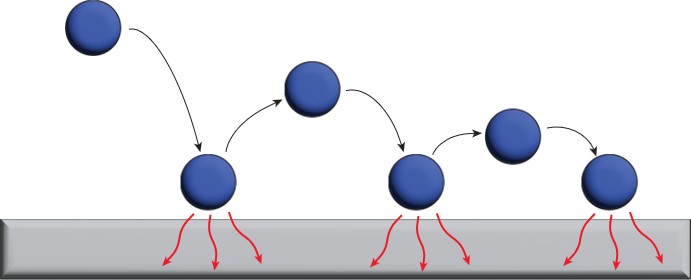
Why does this happen? Let’s consider the same bouncing ball, but instead let’s pretend that energy in the ball can exist only within boxes in the ball and the floor (Figure 1). In the beginning, all the energy is confined to the boxes within the ball. As the ball bounces, some of that energy leaves the ball and is able to disperse to the boxes within the floor. This readily happens because there are more boxes in the floor than in the ball. We can label each of these boxes as a microstate. Simply put, a microstate is one way for molecules in a system can arrange at a given energy.
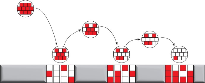
We can consider how entropy changes as a substance undergoes phase transitions. In a solid, all the composite atoms or molecules are tightly held together which prevents them from freely moving around. In a liquid, the composite atoms or molecules are able to move freely around each other, while still being confined to a specific volume. In a gas, all the composite atoms or molecules are able to freely move around each other and are completely free to occupy the entire volume of whatever container the gas is in. From this we can say that a solid has the least entropy (fewest number of microstates), a gas has the most entropy (largest number of microstates), and liquids fall in between the two.
Experiment Overview
During this four-part experiment, you will be tasked with (1) calibrating a coffee cup calorimeter by determining it’s specific heat, (2) determining the specific heat of an unknown metal, (3) determining an overall ΔH using Hess’s Law, and (4) determining change in entropy upon dissolving urea in water. You will complete parts 1, 2, and 3 during the first week, and finish part 4 during the second week.
Safety and Waste Disposal
During this lab, you will be pulling hot water out of a large beaker using a smaller (50 mL) beaker. This should be done using tongs to hold onto the smaller beaker, and with extra care to ensure the hot water does not splash on you. Additionally, there are quite a few temperature fluctuations in this lab, and while the borosilicate glass used in lab glassware is more resistant to thermal shock, care should be taken to avoid shocking the glassware with extreme temperature changes (i.e., do not place a hot piece of glass directly into cold water, or vice versa).
While the majority of chemicals in this lab are fairly benign, there are some concerns that need to be addressed. The unknown metal samples in part 2 must always be handled carefully and with nitrile gloves. Hydrochloric acid is a strong acid and is a corrosion agent that will cause severe eye irritation and damage upon contact. Inhaling the solution vapors may lead to respiratory irritation and should be avoided. You will be using both 1 M and 3 M HCl is this lab, so extra care should be taken while handling the solutions. Should you get any acid on your skin, alert your TA immediately and rinse the affected area under running water for at least 15 minutes. Click here to see the SDS.
Urea is a nitrogen-containing compound that may have a distinct smell. Should the compound come into contact with your skin, alert your TA immediately and flush the area with running water for at least 15 minutes. Inhalation of urea vapors may cause irritation or dizziness. Should you feel respiratory irritation or light-headedness, alert your TA and step out of the lab to get fresh air. You may return to the experiment when you are feeling better. Click here to see the SDS.
In part 1, the water used to determine the specific heat of the coffee cup calorimeter may be disposed of down the sinks. In part 2, the water used in the coffee cups may be disposed of in the sinks, but the metal you used should be placed in the container labelled for wet samples of that type of metal (A, B, C, or D) in the fume hood. Be careful to not mix the metal samples together! Ask your TA for guidance if you’re unsure which container to put the wet metal in. In part 3, the hydrochloric acid solutions should be disposed of in the proper inorganic waste jugs in the fume hood. In part 4, the waste solutions should be discarded in the inorganic waste jugs in the fume hoods, as was done in part 3.
Experimental Procedure
Before beginning, fill a 1000 mL beaker about three-fourths full with ice and add water to make an ice bath. Separately, add about 20 mL of deionized water to two test tubes and cap the test tubes with the provided rubber corks. The exact volume in the test tubes is not important, as you’ll see later. Place the test tubes in the ice bath so that they are cold for part 2!
Part 1: Calibration of the calorimeter
To start, set up your coffee cup calorimeter by stacking two Styrofoam cups in each other. Drop a stirbar into the cups and place a lid on the cup as a cap. Use a top-loading balance to obtain the mass of this setup. Place the calorimeter in a 400 mL beaker, and place this entire setup in a ring clamp so that it cannot tip over. Insert the temperature probe through the hole in the coffee cup lid so that it will be submerged in the liquid, but not so far that it pokes a hole through the inner coffee cup. Add about 40 mL of room temperature DI water to the calorimeter. The exact volume does not matter, because you will then obtain the mass of the setup with the water on the top-loading balance (just the mass of the coffee cups, stirbar, and lid — do not include the beaker). Place the calorimeter in the beaker on the stir plate and turn the stir plate on. At this point, record the temperature of the hot water bath, but do not remove any of the water yet.
To set up the Logger Pro, connect the temperature probe to Channel 1 of the Vernier computer interface and connect the interface to the computer. Open the Logger Pro software, click on “Experiment”, and then click on the “Data Collection” option in the dropdown menu. Change the experiment duration to 600 seconds and the samples/second to 1. Now you can insert the temperature probe into the coffee cup calorimeter (if it isn’t already in the lid) such that the probe is in the room temperature water, but not so far as to touch the bottom of the coffee cup. Click “Collect” on the Logger Pro software to begin the data collection. This will serve as the initial temperature of the water bath.
Using a set of tongs, dip a 50 mL beaker into the hot water bath so that it fills the beaker entirely. Carefully dump out a little of the water back into the hot water batch so that the 50 mL beaker is not overflowing. Quickly, but carefully, add the hot water to the coffee cup calorimeter while the data is collecting (you should have about 2 minutes worth of room temperature data collected at this point). Once the hot water is added to the calorimeter, quickly replace the lid and monitor the temperature for the remaining experiment time. Your temperature should be a constant line or should be steadily, slowly decreasing.
After the data collection time has ended (5 minutes total), obtain the mass of the system again in the same manner as before. This will allow you to determine the exact mass of hot water you added to the system. Once you’ve obtained the new mass, you may dump the water down the sink and carefully dry the entirety of the calorimeter.
Part 2: Determination of the specific heat of an unknown metal
Choose any of the provided unknown metal samples from the fume hood and record the identity of the chosen metal (A, B, C, or D). Weigh out about 100 g of the metal into a 50 mL beaker using a top-loading balance. Be sure to record any and all physical observations regarding the metal! For example, what shape is the metal? Are the pieces spherical, or long strips? Do they pieces of metal have a metallic sheen to them or is there a layer of oxidation? Use the temperature probe to “stir” the metal pieces around in the 50 mL beaker. Record the temperature of the beads to 0.01°C.
Remember those two test tubes you placed in the ice bath at the beginning of the lab? Grab both of those and wipe off the outsides of the tubes before pouring the cold water into the calorimeter. Replace the cap of the calorimeter, turn on the stirring and allow the water to stir for about 3 seconds, then click the “Collect” button on the Logger Pro software. After recording the temperature for about 1 minute, add all of the metal pellets at the same time, but be careful to not splash any of the water! We will need an accurate mass after the data collection period, so you must be careful to not lose any of the water!
Tips and Tricks: It’s important that the mixture in the calorimeter is stirring. If the stirbar is having trouble moving because of all the metal pieces, you may gently use the temperature probe to stir the pellets around. If you must do this, be extra careful that you don’t accidentally puncture the inner coffee cup!
After collecting temperature data for another three minutes, click the “Stop” button to end the data collection. Obtain the mass of the calorimeter on the top-loading balance as you have previously done. This should give you three separate mass values for part 2: an empty calorimeter mass (you may have only collected this at the beginning of part 1), the mass of the metal pieces, and the final mass of the calorimeter, metal pieces, and water. You can then determine the exact mass of the water added by subtracting the mass of the empty calorimeter + the mass of the metal pieces from the final mass.
After obtaining the final mass, you may dispose of the sample as described in the Safety and Waste section of the pre-lab reading. Carefully dry the entirety of the coffee cup calorimeter and move on to Part 3.
Part 3: Determination of the heat of formation of MgO
First, obtain a pre-cut strip of magnesium ribbon from the supplies bench along with a piece of sandpaper. You should notice that there is an uneven layer of black material on the surface of the strip. This is the oxide layer on the ribbon, so you need to carefully sand off the oxide layer. DO NOT sand directly on the benchtops, as this can permanently damage the surface of the benches. Once the magnesium strip appears silver and shiny, obtain the mass using an analytical balance (the pre-cut strips should be about 120 mg).
Obtain the empty mass of your calorimeter setup using the top-loading balance. Next, get about 30 mL of the 1 M HCl from the fume hood using a clean and dry 50 mL beaker. Add the HCl to the calorimeter and obtain the mass on the top-loading balance again. Set the calorimeter on the stir plate, start stirring, and click “Collect” on the Logger Pro software. After about 2 minutes, loosen the cap of the calorimeter, carefully drop in the pre-weighed strip of magnesium, and replace the calorimeter lid. Allow the Logger Pro to collect the remaining data for the run, which will be approximately 3 more minutes. The data collected by the Logger Pro should be analyzed according to the “Data Manipulation” section below. The solution should be discarded in the inorganic waste jug in the fume hood. Rinse the calorimeter with DI water and carefully dry it with a paper towel.
Now we will repeat this procedure with some slight modifications. Obtain an empty mass of the calorimeter on the top-loading balance. Obtain about 30 mL of 3 M HCl from the fume hood using a 50 mL beaker, add the HCl to the calorimeter, and obtain another mass for the filled calorimeter using the top-loading balance. Separately, obtain the magnesium oxide powder from the fume hood and weigh out about 200 mg onto a weigh boat using an analytical balance. Don’t forget to write down every digit displayed on the balance!
Tips and Tricks: It is a good idea to record the mass of the empty weigh boat before adding any magnesium oxide to the boat (we can call this mboat for the sake of the example). MgO is mildly hygroscopic, so it’s possible that you won’t be able to add in all of the MgO that you initially weighed out. In this case, you can obtain a new mass for the weigh boat that has some of the MgO still on it (mdirty). By subtracting mboat from mdirty, you are left with the mass of MgO that did not make it into the calorimeter. It is important, then, to subtract that mass from the mass of MgO you initially weighed out so that you know exactly how much MgO is in your calorimeter.
As you did previously, start stirring the 3 M HCl solution and click “Collect” on the Logger Pro software to get an initial temperature of the HCl. After about 2 minutes, loosen the calorimeter lid and carefully add in as much of the MgO as possible. While you will ideally get all of the MgO into the calorimeter, it’s likely that some of it will stick to the weigh boat. DO NOT rinse the weigh boat into the calorimeter, as that will add water to the system and alter the results. Replace the calorimeter lid and allow the data collection to finish out, about another 3 minutes. The data collected by the Logger Pro should be analyzed according to the “Data Manipulation” section below. The solution should be discarded in the inorganic waste jug in the fume hood. Rinse the calorimeter with DI water and carefully dry it with a paper towel.
This is the end of the first lab session for Thermochemistry. If you have any remaining time, conduct a second trial for each part of the experiment starting with Part 2.
Part 4: Measuring the change in entropy associated with the dissolution of urea
Begin by setting up your calorimeter as you did for the previous parts. Take a few minutes to make sure that everything is clean and dry! Obtain an empty, dry mass of the calorimeter (including the stirbar) using a top-loading balance. Next, use a graduated cylinder to measure out 50.0 mL of DI water and add that to the calorimeter. It is important that you record a true volume! It’s okay if you added 49.7 mL, just make sure you record it properly. Close the lid of the calorimeter and begin collecting data using the Logger Pro.
While the temperature is collecting, obtain a vial of urea from the fume hood and weigh out 2–3 g into a weigh boat using a top-loading balance. After collecting about 2 minutes of temperature data for the DI water, loosen the calorimeter lid and carefully add in the urea while the system is stirring. Since you are adding a large amount of solid, it’s a good idea to occasionally check to make sure that the stir bar is still spinning. Once the urea is completely dissolved, record the final temperature immediately! Finally, obtain the mass of the entire calorimeter system as you did previously so that you can get an accurate mass of the solution. Once you have recorded the final mass, you may dispose of the entire solution in the inorganic waste jug in the fume hood. Rinse the calorimeter with DI water and carefully dry it with a paper towel.
Now we will conduct a similar experiment using slightly different methods. To start, weigh out 3–5 g of urea on the top-loading balance and add it all to a clean and dry 25 mL graduated cylinder. Note that the urea should be the only thing in the cylinder at this point! It is recommended that you use a clamp to hold onto the graduated cylinder so that you don’t accidentally tip it over in the coming steps.
Using a Pasteur pipette, slowly add 2–3 mL of DI water to the graduated cylinder containing the urea and gently stir it all using the temperature probe. Stir carefully so that you don’t accidentally break the cylinder! Click “Collect” on the Logger Pro to begin collecting temperature data.
Once you’ve added 3 mL of DI water, begin adding more DI water dropwise until the urea has just dissolved. In other words, add DI water dropwise until the moment you no longer see any solid urea, then do not add any more! After the urea has just dissolved, record the final temperature of the solution. Finally, remove the temperature probe and record the final volume of the solution. Once these values have been obtained, you may discard the solution in the inorganic waste jug in the fume hood.
Tips and Tricks: If the urea is taking a long time to dissolve, you may put the cylinder in a beaker of warm water. If you are using this trick, you must keep the water bath around 25°C, and you must ensure that absolutely no water from the water bath gets into the cylinder.
Data Manipulation
The following information regards how to use the Logger Pro and how to properly analyze the data obtained so that you get the proper data from your experiments. First, connect a temperature probe to channel 1 of the Vernier computer interface, and connect the interface to the computer through the USB cable. Open the Logger Pro software, click the “Experiment” menu in the top left of the screen, and click on the “Data Collection” option in the dropdown menu. Change the duration of the experiment to 600 seconds and the samples/second to 1.
Set up the calorimeter as outlined in each section above. Once you are ready, click “Collect” on the Logger Pro to begin the data collection. This will give you the initial temperature of the water or HCl solution. Once the temperature is stable and data has been collected for about 2 minutes, add in the appropriate material depending on which part of the experiment you are doing (hot water, MgO, etc.). Be sure to add in all of the material at once without splashing any water and immediately close the lid again. Note that the stirbar should be constantly stirring. Data will automatically be collected for 10 minutes, but you may hit the “Stop” button if the temperature has plateaued or if the temperature has begun a steady, linear decrease over a period of a few minutes.
Once data collection has stopped, select the point of maximum temperature and drag the cursor to the end of the data on the right-hand side of the plot. Essentially, you are trying to highlight the linear region of the plot. Click on the “Linear Fit” icon along the top toolbar of the plot window. This should add a linear fit to the highlighted portion of the plot that includes the slope and y-intercept of the fit line. Record the slope and y-intercept in your lab notebook.
Now you can use that line equation to extrapolate your Tf value. The Tf value is the temperature that the system would have reached if everything had been mixed instantaneously and absolutely no heat was lost. Of course, we know that this is a very idealized circumstance, but we can predict what that value would be based on the linear fit of the plot. Find the exact time that you added in the new material and plug that into the linear fit equation. Solving the equation for y at this time will give the temperature T at the time of mixing. Record the initial temperature (at the time of mixing) and the extrapolated temperature in your data table. Be sure to label them carefully so that you do not get them confused during your data workup.
The process of dissolving a solid (solute) in a liquid solvent.
The sum of a system's internal energy (U) and the product of the pressure (P) and volume (V). Mathematically represented as
H = U + PV
A type of a reaction that absorbs heat from the surroundings, typically the solvent. This makes the temperature of the mixture decrease, since the solvent makes up the immediate surroundings.
A type of reaction in which heat is lost from the system to the surroundings. This makes the temperature of the mixture increase, since the solvent makes up the immediate surroundings.
A function whose value depends only on the initial and finals states rather than the path(s) taken to get there.
Enthalpy associated with a solute dissolving into a solvent.
A measure of how resistant a substance is to changes in temperature. It is often represented by C.
A description of how molecules may arrange at a given energy. Often related to entropy, systems with more microstates have greater entropy.
If a material is hygroscopic, it will readily absorb water from the surrounding air. Materials that are highly hygroscopic may even absorb enough water to cause them to dissolve!