
1.6 Transformations
Theorems 1.4, 2.1, 2.2, 3.1, 4.1 and 4.4 all describe ways in which the graph of a function can changed, or transformed to obtain the graph of a related function. The results and proofs of each of these theorems are virtually identical, and with the language of function composition, we can see better why.
Consider, for instance, Theorem 4.4, in which we will describe how to transform the graph of [latex]f(x) = x^r[/latex] to [latex]F(x) = a(bx-h)^r +k[/latex]. We may think of [latex]F[/latex] as being build up from [latex]f[/latex] by composing [latex]f[/latex] with linear functions. Specifically, if we let [latex]i(x) = bx-h[/latex], then [latex](f\circ i)(x) = f(i(x)) = f(bx-h) = (bx-h)^r[/latex]. If, additionally, we let and [latex]j(x) = ax+k[/latex], then [latex](j \circ (f \circ i))(x) = j( (f \circ i)(x)) = j((bx-h)^r) = a(bx-h)^r+k = F(x)[/latex]. Hence, we can view [latex]F = j \circ f \circ i[/latex].
In this section, our goal is to generalize the aforementioned theorems to the graphs of all functions. Along the way, you’ll see some very familiar arguments, but, additionally, we hope this section affords the reader an opportunity to not only see how these transformations work they way they do, but why.
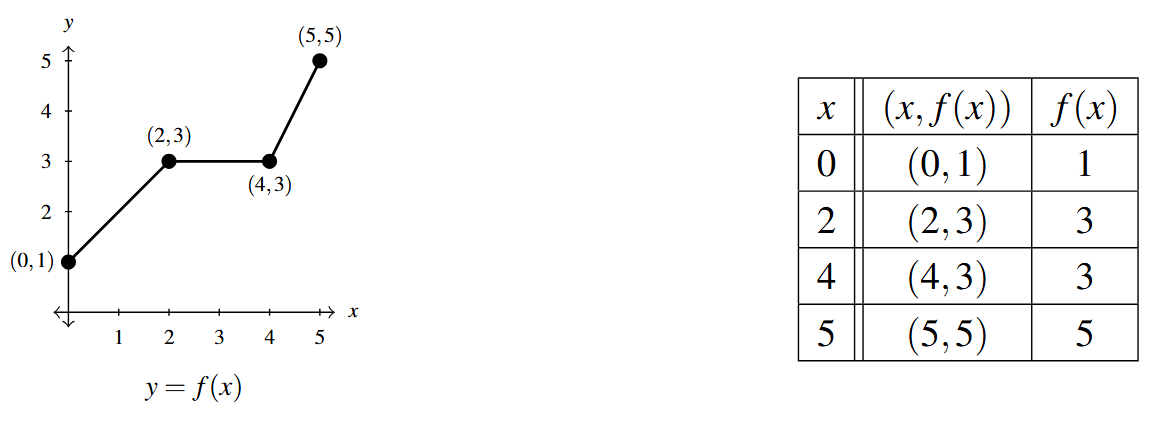
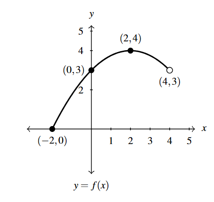
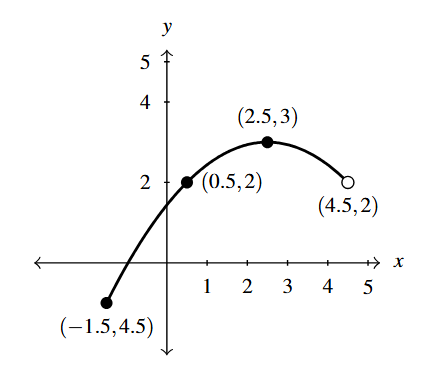
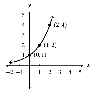
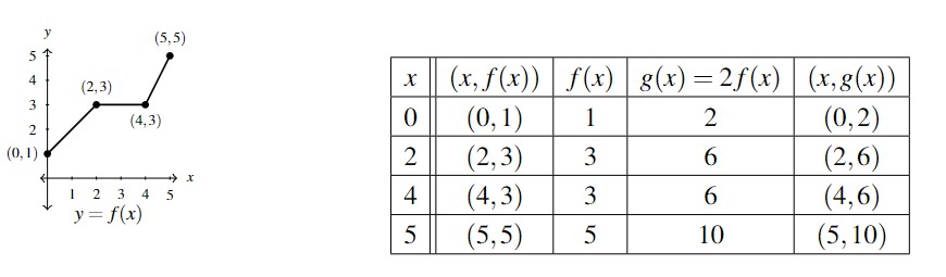
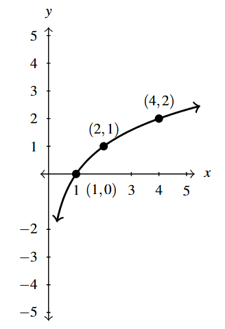
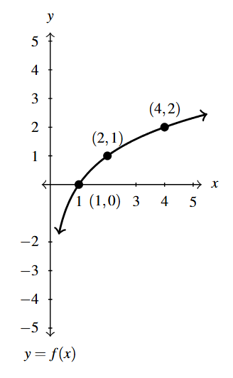
Our motivational example for the results in this section is the graph of [latex]y = f(x)[/latex] below. While we could formulate an expression for [latex]f(x)[/latex] as a piecewise-defined function consisting of linear and constant parts, we wish to focus more on the geometry here. That being said, we do record some of the function values – the key points if you will – to track through each transformation.
1.6.1 Vertical and Horizontal Shifts
Suppose we wished to graph [latex]g(x) = f(x) + 2[/latex]. From a procedural point of view, we start with an input [latex]x[/latex] to the function [latex]f[/latex] and we obtain the output [latex]f(x)[/latex]. The function [latex]g[/latex] takes the output [latex]f(x)[/latex] and adds 2 to it. Using the sample values for [latex]f[/latex] from the table above we can create a table of values for [latex]g[/latex] below, hence generating points on the graph of [latex]g[/latex].
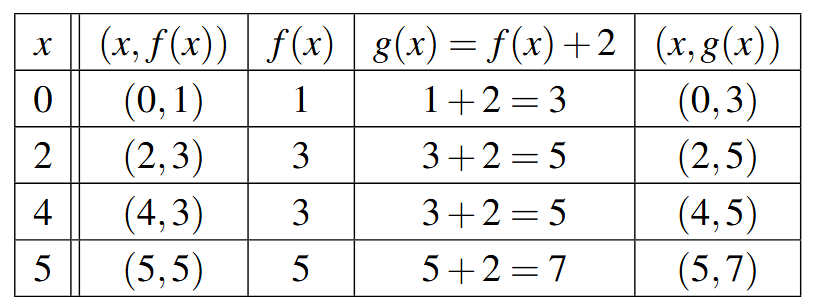
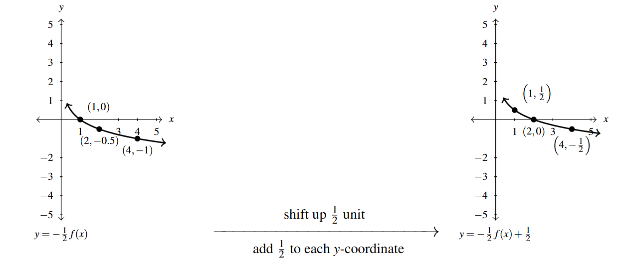
In general, if [latex](a,b)[/latex] is on the graph of [latex]y=f(x)[/latex], then [latex]f(a) = b[/latex]. Hence, [latex]g(a) = f(a) +2 = b+2[/latex], so the point [latex](a,b+2)[/latex] is on the graph of [latex]g[/latex]. In other words, to obtain the graph of [latex]g[/latex], we add 2 to the [latex]y[/latex]-coordinate of each point on the graph of [latex]f[/latex].
Geometrically, adding 2 to the [latex]y[/latex]-coordinate of a point moves the point 2 units above its previous location. Adding 2 to every [latex]y[/latex]-coordinate on a graph en masse is moves or shifts the entire graph of [latex]f[/latex] up 2 units. Notice that the graph retains the same basic shape as before, it is just 2 units above its original location. In other words, we connect the four key points we moved in the same manner in which they were connected before.
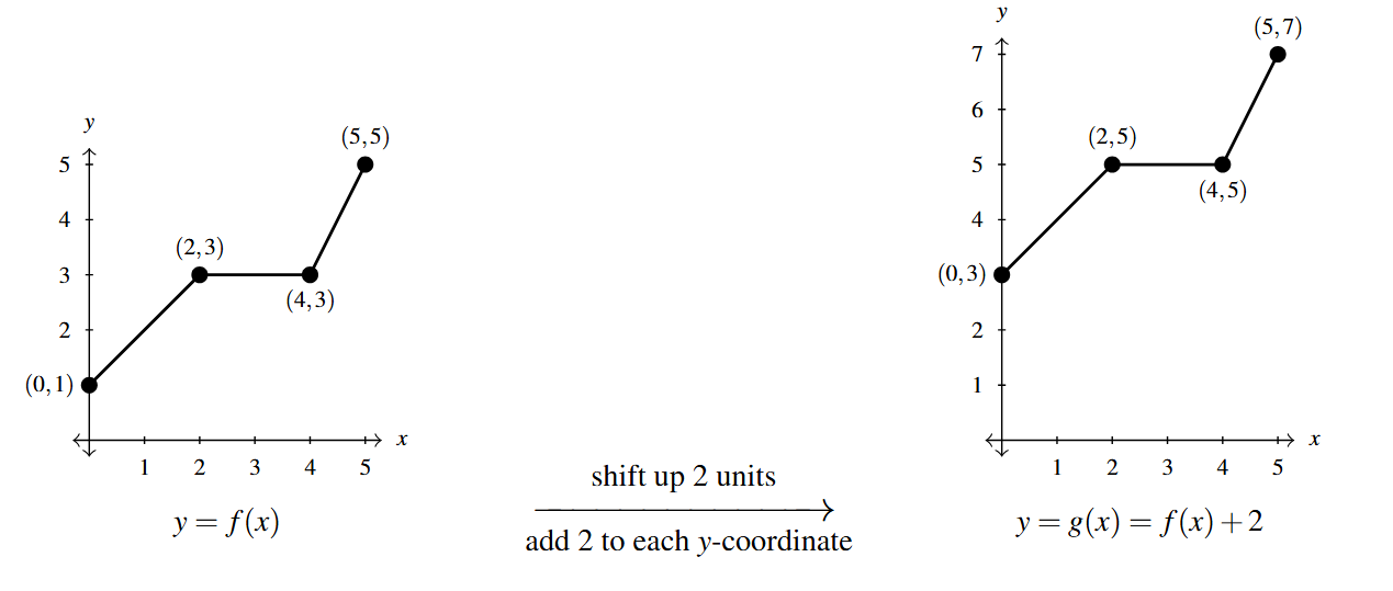
You’ll note that the domain of [latex]f[/latex] and the domain of [latex]g[/latex] are the same, namely [latex][0,5][/latex], but that the range of [latex]f[/latex] is [latex][1,5][/latex] while the range of [latex]g[/latex] is [latex][3,7][/latex]. In general, shifting a function vertically like this will leave the domain unchanged, but could very well affect the range.
You can easily imagine what would happen if we wanted to graph the function [latex]j(x) = f(x) - 2[/latex]. Instead of adding 2 to each of the [latex]y[/latex]-coordinates on the graph of [latex]f[/latex], we’d be subtracting 2. Geometrically, we would be moving the graph down 2 units. We leave it to the reader to verify that the domain of [latex]j[/latex] is the same as [latex]f[/latex], but the range of [latex]j[/latex] is [latex][-1,3][/latex]. In general, we have:
Suppose [latex]f[/latex] is a function and [latex]k[/latex] is a real number
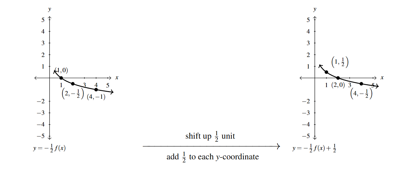
To graph [latex]F(x) = f(x) + k[/latex], add [latex]k[/latex] to each of the [latex]y[/latex]-coordinates of the points on the graph of [latex]y=f(x)[/latex].
NOTE: This results in a vertical shift up [latex]k[/latex] units if [latex]k > 0[/latex] or down [latex]k[/latex] units if [latex]k[/latex] < [latex]0[/latex].
To prove Theorem 1.7, we first note that [latex]f[/latex] and [latex]F[/latex] have the same domain (why?) Let [latex]c[/latex] be an element in the domain of [latex]F[/latex] and, hence, the domain of [latex]f[/latex]. The fact that [latex]f[/latex] and [latex]F[/latex] are functions guarantees there is exactly one point on each of their graphs corresponding to [latex]x=c[/latex]. On [latex]y=f(x)[/latex], this point is [latex](c, f(c))[/latex]; on [latex]y = F(x)[/latex], this point is [latex](c, F(c)) = (c, f(c)+k)[/latex]. This sets up a nice correspondence between the two graphs and shows that each of the points on the graph of [latex]F[/latex] can be obtained to by adding [latex]k[/latex] to each of the [latex]y[/latex]-coordinates of the corresponding point on the graph of [latex]f[/latex]. This proves Theorem 1.7. In the language of inputs and outputs, Theorem 1.7 says adding to the output of a function causes the graph to shift vertically.
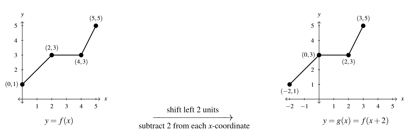
Keeping with the graph of [latex]y=f(x)[/latex] above, suppose we wanted to graph [latex]g(x) = f(x+2)[/latex]. In other words, we are looking to see what happens when we add 2 to the input of the function. Let’s try to generate a table of values of [latex]g[/latex] based on those we know for [latex]f[/latex]. We quickly find that we run into some difficulties. For instance, when we substitute [latex]x=4[/latex] into the formula [latex]g(x)=f(x+2)[/latex], we are asked to find [latex]f(4+2)=f(6)[/latex] which doesn’t exist because the domain of [latex]f[/latex] is only [latex][0,5][/latex]. The same thing happens when we attempt to find [latex]g(5)[/latex].
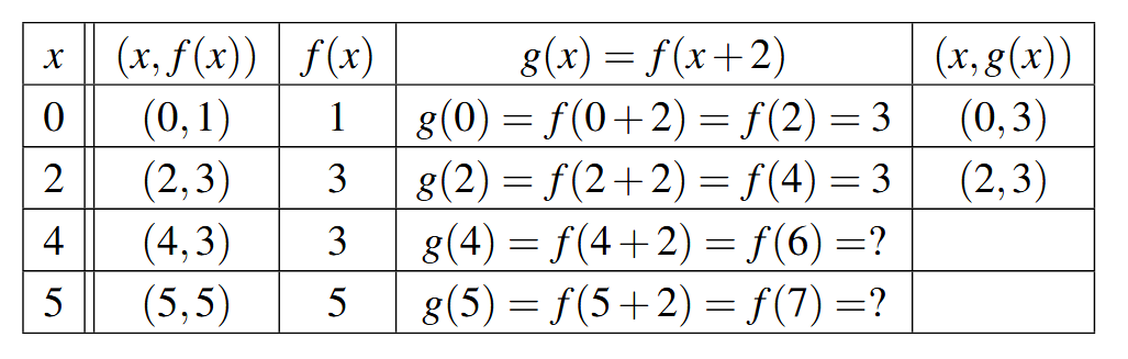
What we need here is a new strategy. We know, for instance, [latex]f(0) = 1[/latex]. To determine the corresponding point on the graph of [latex]g[/latex], we need to figure out what value of [latex]x[/latex] we must substitute into [latex]g(x) = f(x+2)[/latex] so that the quantity [latex]x+2[/latex], works out to be 0. Solving [latex]x+2=0[/latex] gives [latex]x=-2[/latex], and [latex]g(-2) = f((-2)+2) = f(0) = 1[/latex] so [latex](-2,1)[/latex] on the graph of [latex]g[/latex]. To use the fact [latex]f(2) = 3[/latex], we set [latex]x+2 = 2[/latex] to get [latex]x=0[/latex]. Substituting gives [latex]g(0) = f(0+2) = f(2) = 3[/latex]. Continuing in this fashion, we produce the table below.
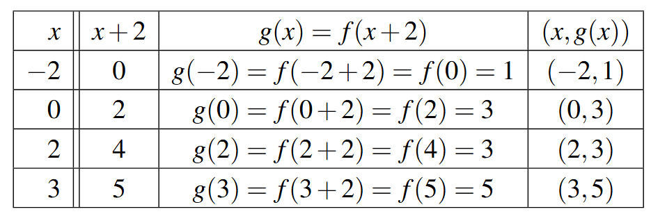
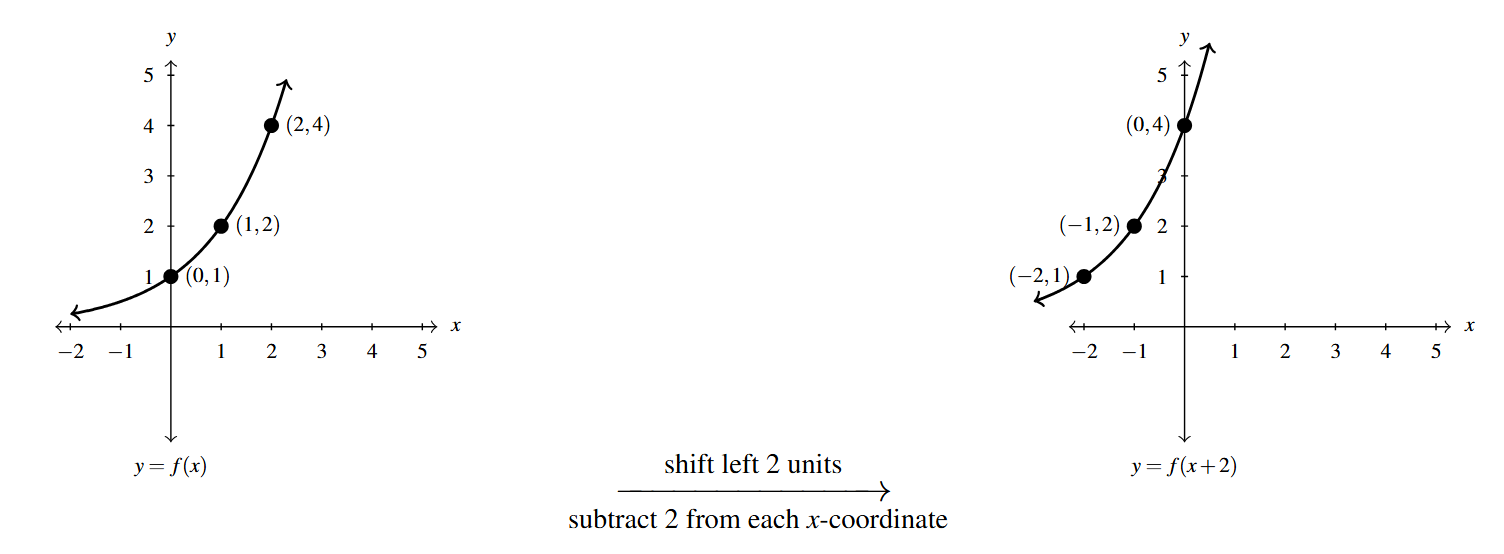
In summary, the points [latex](0,1)[/latex], [latex](2,3)[/latex], [latex](4,3)[/latex] and [latex](5,5)[/latex] on the graph of [latex]y=f(x)[/latex] give rise to the points [latex](-2,1)[/latex], [latex](0,3)[/latex], [latex](2,3)[/latex] and [latex](3,5)[/latex] on the graph of [latex]y=g(x)[/latex], respectively. In general, if [latex](a,b)[/latex] is on the graph of [latex]y=f(x)[/latex], then [latex]f(a) = b[/latex]. Solving [latex]x+2 = a[/latex] gives [latex]x = a-2[/latex] so that [latex]g(a-2) = f((a-2)+2) = f(a) = b[/latex]. As such, [latex](a-2,b)[/latex] is on the graph of [latex]y=g(x)[/latex]. The point [latex](a-2,b)[/latex] is exactly 2 units to the \emph{left} of the point [latex](a,b)[/latex] so the graph of [latex]y=g(x)[/latex] is obtained by shifting the graph [latex]y=f(x)[/latex] to the left 2 units, as pictured below.
Note that while the ranges of [latex]f[/latex] and [latex]g[/latex] are the same, the domain of [latex]g[/latex] is [latex][-2,3][/latex] whereas the domain of [latex]f[/latex] is [latex][0,5][/latex]. In general, when we shift the graph horizontally, the range will remain the same, but the domain could change. If we set out to graph [latex]j(x) = f(x-2)[/latex], we would find ourselves adding 2 to all of the [latex]x[/latex] values of the points on the graph of [latex]y=f(x)[/latex] to effect a shift to the right 2 units. Generalizing these notions produces the following result.
To prove Theorem 1.8, we first note the domains of [latex]f[/latex] and [latex]F[/latex] may be different. If [latex]c[/latex] is in the domain of [latex]f[/latex], then the only number we know for sure is in the domain of [latex]F[/latex] is [latex]c+h[/latex], due to [latex]F(c+h) = f((c+h)-h) = f(c)[/latex]. This sets up a nice correspondence between the domain of [latex]f[/latex] and the domain of [latex]F[/latex] which spills over to a correspondence between their graphs, The point [latex](c, f(c))[/latex] is the one and only point on the graph of [latex]y = f(x)[/latex] corresponding to [latex]x=c[/latex] just as the point [latex](c+h, F(c+h)) = (c+h, f(c))[/latex] is the one and only point on the graph of [latex]y = F(x)[/latex] corresponding to [latex]x=c+h[/latex]. This correspondence shows we may obtain the graph of [latex]F[/latex] by adding [latex]h[/latex] to each [latex]x[/latex]-coordinate of each point on the graph of [latex]f[/latex], which establishes the theorem. In words, Theorem 1.8 says that subtracting from the input to a function amounts to shifting the graph horizontally.
Theorems 1.7 and 1.8 present a theme which will run common throughout the section: changes to the outputs from a function result in some kind of vertical change; changes to the inputs to a function result in some kind of horizontal change. We demonstrate Theorems 1.7 and 1.8 in the example below.
Example 1.6.1
Example 1.6.1.1a
Use Theorems 1.7 and 1.8 to answer the questions below. Check your answers using a graphing utility where appropriate.
Suppose [latex](-1,3)[/latex] is on the graph of [latex]y = f(x)[/latex]. State a point on the graph of:
[latex]y = f(x)+5[/latex]
Solution:
Suppose [latex](-1,3)[/latex] is on the graph of [latex]y = f(x)[/latex]. State a point on the graph of [latex]y=f(x)+5[/latex].
To apply Theorem 1.7, we identify [latex]f(x)+5 = f(x)+k[/latex] so [latex]k = 5[/latex].
Hence, we add [latex]5[/latex] to the [latex]y[/latex]-coordinate of [latex](-1,3)[/latex] and get [latex](-1,3+5) = (-1,8)[/latex].
To check our answer note that [latex](-1,3)[/latex] is on the graph of [latex]f[/latex] means [latex]f(-1) = 3[/latex]. Substituting [latex]x=-1[/latex] into the formula [latex]y = f(x)+5[/latex], we get [latex]y = f(-1)+5 = 3+5 = 8[/latex].
Hence, [latex](-1,8)[/latex] is on the graph of [latex]f(x)+5[/latex].
Example 1.6.1.1b
Use Theorems 1.7 and 1.8 to answer the questions below. Check your answers using a graphing utility where appropriate.
Suppose [latex](-1,3)[/latex] is on the graph of [latex]y = f(x)[/latex]. State a point on the graph of:
[latex]y = f(x+5)[/latex]
Solution:
Suppose [latex](-1,3)[/latex] is on the graph of [latex]y = f(x)[/latex]. State a point on the graph of [latex]y=f(x+5)[/latex].
We note that [latex]f(x+5)[/latex] can be written as [latex]f(x-(-5)) = f(x-h)[/latex] so we apply Theorem 1.8 with [latex]h=-5[/latex].
Adding [latex]-5[/latex] to (subtracting [latex]5[/latex] from) the [latex]x[/latex]-coordinate of [latex](-1,3)[/latex] gives [latex](-1+(-5), 3) = (-6,3)[/latex].
To check our answer, [latex](-1,3)[/latex] is on the graph of [latex]f[/latex], thus [latex]f(-1) = 3[/latex]. Substituting [latex]x=-6[/latex] into [latex]y=f(x+5)[/latex] gives [latex]y=f(-6+5)=f(-1)=3[/latex], proving [latex](-6,3)[/latex] is on the graph of [latex]y=f(x+5)[/latex].
Example 1.6.1.1c
Use Theorems 1.7 and 1.8 to answer the questions below. Check your answers using a graphing utility where appropriate.
Suppose [latex](-1,3)[/latex] is on the graph of [latex]y = f(x)[/latex]. State a point on the graph of:
[latex]f(x-7)+4[/latex]
Solution:
Suppose [latex](-1,3)[/latex] is on the graph of [latex]y = f(x)[/latex]. State a point on the graph of [latex]y=f(x-7)+4[/latex].
Note that the expression [latex]f(x-7)+4[/latex] differs from [latex]f(x)[/latex] in two ways indicating two different transformations. In situations like this, its best if we handle each transformation in turn, starting with the graph of [latex]y=f(x)[/latex] and building up to the graph of [latex]y = f(x-7)+4[/latex].
We choose to work from the inside (argument) out and use Theorem 1.8 to first get a point on the graph of [latex]y=f(x-7) = f(x-h)[/latex]. Identifying [latex]h=7[/latex], we add [latex]7[/latex] to the [latex]x[/latex]-coordinate of [latex](-1,3)[/latex] to get [latex](-1+7,3) = (6,3)[/latex]. Hence, [latex](6,3)[/latex] is a point on the graph of [latex]y = f(x-7)[/latex].
Next, we apply Theorem 1.7 to graph [latex]y = f(x-7)+4[/latex] starting with [latex]y=f(x-7)[/latex]. Viewing [latex]f(x-7)+4 = f(x-7)+k[/latex], we identify [latex]k=4[/latex] and add [latex]4[/latex] to the [latex]y[/latex]-coordinate of [latex](6,3)[/latex] to get [latex](6,3+4) = (6,7)[/latex].
To check, we note that if we substitute [latex]x=6[/latex] into [latex]y = f(x-7)+4[/latex], we get [latex]y=f(6-7)+4 = f(-1)+4 = 3+4 =7[/latex].
Example 1.6.1.2a
Use Theorems 1.7 and 1.8 to answer the questions below. Check your answers using a graphing utility where appropriate.
Write a formula for a function [latex]g(t)[/latex] whose graph is the same as [latex]f(t) = |t|-2t[/latex] but is shifted:
to the right [latex]4[/latex] units.
Solution:
Here the independent variable is [latex]t[/latex] instead of [latex]x[/latex] which doesn’t affect the geometry in any way as our convention is the independent variable is used to label the horizontal axis and the dependent variable is used to label the vertical axis.
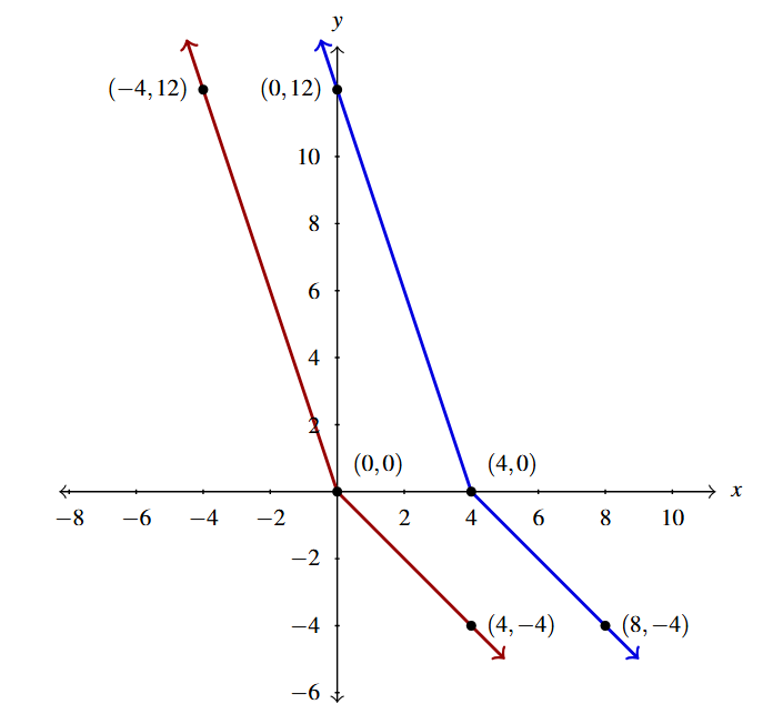
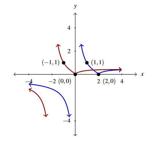
Write a formula for a function [latex]g(t)[/latex] whose graph is the same as [latex]f(t) = |t|-2t[/latex] but is shifted to the right 4 units.
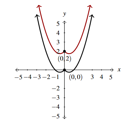
Per Theorem 1.8, the graph of [latex]g(t) = f(t-4) = |t-4|-2(t-4) = |t-4|-2t+8[/latex] (in blue) should be the graph of [latex]f(t) = |t|-2t[/latex] (in red) shifted to the right [latex]4[/latex] units.
Our check is below.
Example 1.6.1.2b
Use Theorems 1.7 and 1.8 to answer the questions below. Check your answers using a graphing utility where appropriate.
Write a formula for a function [latex]g(t)[/latex] whose graph is the same as [latex]f(t) = |t|-2t[/latex] but is shifted:
down 2 units.
Solution:
Here the independent variable is [latex]t[/latex] instead of [latex]x[/latex] which doesn’t affect the geometry in any way as our convention is the independent variable is used to label the horizontal axis and the dependent variable is used to label the vertical axis.
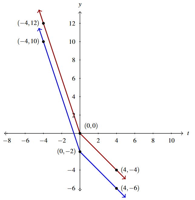
Write a formula for a function [latex]g(t)[/latex] whose graph is the same as [latex]f(t) = |t|-2t[/latex] but is shifted to the down 2 units.
Per Theorem 1.7, the graph of [latex]g(t) = f(t)+(-2) = |t|-2t+(-2) = |t|-2t-2[/latex] (in blue) should be the graph of [latex]f(t) = |t|-2t[/latex] (in red) shifted down 2 units.
Our check is below.
Example 1.6.1.3
Use Theorems 1.7 and 1.8 to answer the questions below. Check your answers using a graphing utility where appropriate.
Predict how the graph of [latex]F(x) = \dfrac{(x-2)^{\frac{2}{3}}}{x}[/latex] relates to the graph of [latex]f(x) = \dfrac{x^{\frac{2}{3}}}{x+2}[/latex].
Solution:
Predict how the graph of [latex]F(x) = \dfrac{(x-2)^{\frac{2}{3}}}{x}[/latex] relates to the graph of [latex]f(x) = \dfrac{x^{\frac{2}{3}}}{x+2}[/latex].
Comparing formulas, it appears as if [latex]F(x) = f(x-2)[/latex]. We check: \[ \begin{array}{rcl} f(x-2) &=& \dfrac{(x-2)^{\frac{2}{3}}}{(x-2)+2}\\ &=& \dfrac{(x-2)^{\frac{2}{3}}}{x}\\ &=& F(x), \end{array} \] so, per Theorem 1.8, the graph of [latex]y = F(x)[/latex] (in blue) should be the graph of [latex]y=f(x)[/latex] (in red) but shifted to the right 2 units.
We graph both functions below to confirm our answer.
Example 1.6.1.4a
Use Theorems 1.7 and 1.8 to answer the questions below. Check your answers using a graphing utility where appropriate.
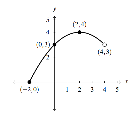
Below on is the graph of [latex]y = f(x)[/latex].
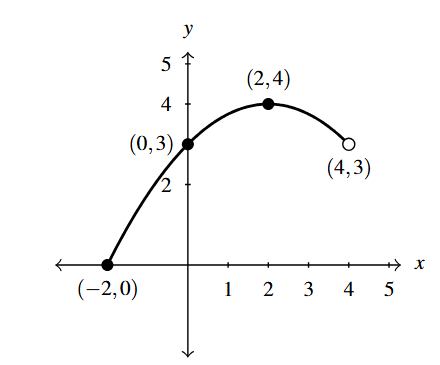
Use it to sketch the graph of
[latex]F(x) = f(x-2)[/latex]
Solution:
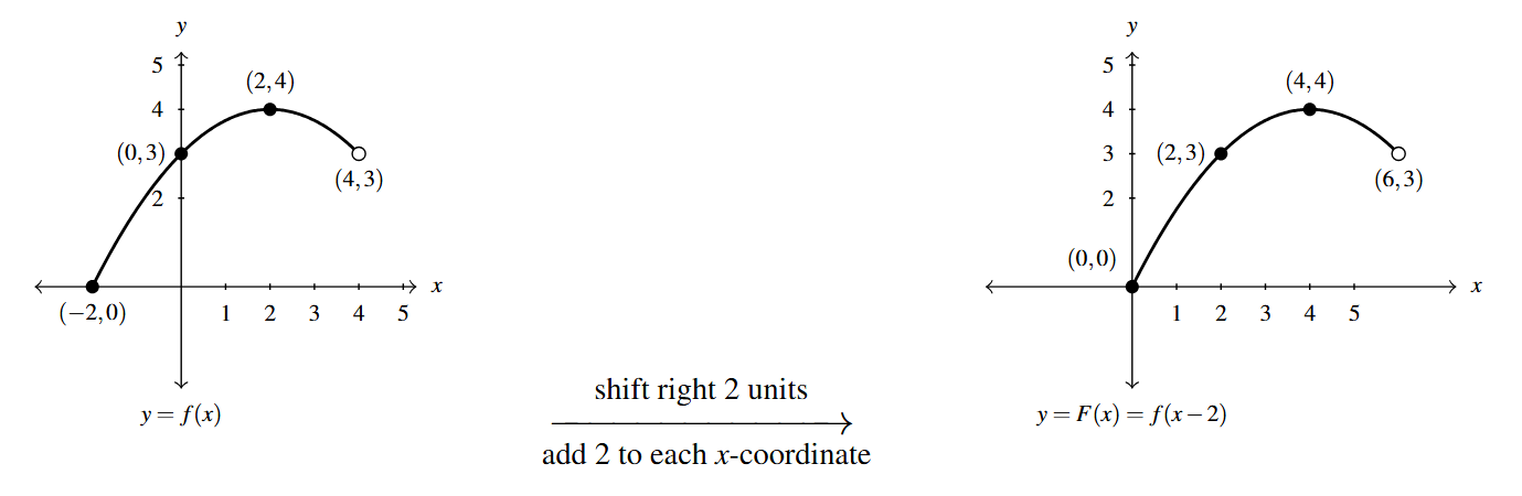
Sketch a graph of [latex]F(x) = f(x-2)[/latex].
We recognize [latex]F(x) = f(x-2) =f(x-h)[/latex]. With [latex]h=2[/latex], Theorem 1.8 tells us to add 2 to each of the [latex]x[/latex]-coordinates of the points on the graph of [latex]f[/latex], moving the graph of [latex]f[/latex] to the right two units.
We can check our answer by showing each ordered pair [latex](x,y)[/latex] listed on our final graph satisfies the equation [latex]y = f(x-2)[/latex].
Starting with [latex](0,0)[/latex], we substitute [latex]x=0[/latex] into [latex]y=f(x-2)[/latex] and get [latex]y = f(0-2) = f(-2)[/latex]. [latex](-2,0)[/latex] is on the graph of [latex]f[/latex], so we know [latex]f(-2) = 0[/latex]. Hence, [latex]y = f(0-2) = f(-2) = 0[/latex], showing the point [latex](0,0)[/latex] is on the graph of [latex]y=f(x-2)[/latex]. We invite the reader to check the remaining points.
Example 1.6.1.4b
Use Theorems 1.7 and 1.8 to answer the questions below. Check your answers using a graphing utility where appropriate.
Below on is the graph of [latex]y = f(x)[/latex].
Use it to sketch the graph of
[latex]F(x)= f(x)+1[/latex]
Solution:
Sketch a graph of [latex]F(x) = f(x)+1[/latex].
We have [latex]F(x) = f(x)+1 = f(x)+k[/latex] where [latex]k=1[/latex], so Theorem 1.7 tells us to move the graph of [latex]f[/latex] up 1 unit by adding 1 to each of the [latex]y[/latex]-coordinates of the points on the graph of [latex]f[/latex].
To check our answer, we proceed as above. Starting with the point [latex](-2,1)[/latex], we substitute [latex]x=-2[/latex] into [latex]y=f(-2)+1[/latex] to get [latex]y = f(-2)+1[/latex]. Given [latex](-2,0)[/latex] is on the graph of [latex]f[/latex], we know [latex]f(-2) = 0[/latex]. Hence, [latex]y = f(-2)+1 =0+1 = 1[/latex]. This proves [latex](-2,1)[/latex] is on the graph of [latex]y=f(x)+1[/latex]. We encourage the reader to check the remaining points in kind.
Example 1.6.1.4c
Use Theorems 1.7 and 1.8 to answer the questions below. Check your answers using a graphing utility where appropriate.
Below on is the graph of [latex]y = f(x)[/latex].
Use it to sketch the graph of
[latex]F(x)= f(x+1)-2[/latex]
Solution:
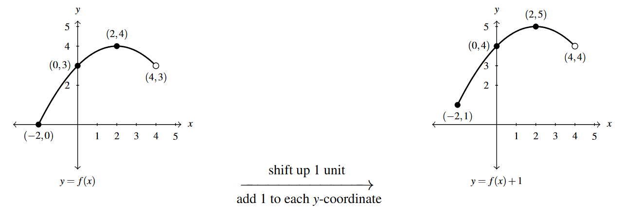
Sketch a graph of [latex]F(x) = f(x+1)-2[/latex].
We are asked to graph [latex]F(x) = f(x+1) -2[/latex]. As above, when we have more than one modification to do, we work from the inside out and build up to [latex]F(x)=f(x+1)-2[/latex] from [latex]f(x)[/latex] in stages.
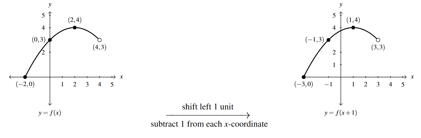
First, we apply Theorem 1.8 to graph [latex]y=f(x+1)[/latex] from [latex]y=f(x)[/latex]. Rewriting [latex]f(x+1) = f(x-(-1))[/latex], we identify [latex]h=-1[/latex], so we add [latex]-1[/latex] to (subtract 1 from) each of the [latex]x[/latex]-coordinates on the graph of [latex]f[/latex], shifting it to the left 1 unit.
Next, we apply Theorem 1.7 to graph [latex]y = f(x+1)-2[/latex] starting with the graph of [latex]y=f(x+1)[/latex]. Writing [latex]f(x+1)-2=f(x+1)+(-2) = f(x+1)+k[/latex], we identify [latex]k=-2[/latex] so Theorem 1.7 instructs us to add [latex]-2[/latex] to (subtract 2 from) each of the [latex]y[/latex]-coordinates on the graph of [latex]y = f(x+1)[/latex], thereby shifting the graph down two units.
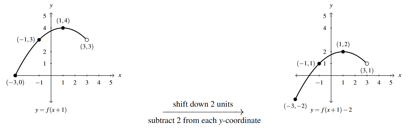
To check, we start with the point [latex](-3, -2)[/latex]. We find when we substitute [latex]x=-3[/latex] into the equation [latex]y=f(x+1)-2[/latex] we get [latex]y = f(-3+1)-2 = f(-2)-2[/latex]. Given [latex](-2,0)[/latex] is on the graph of [latex]f[/latex], we know [latex]f(-2) =0[/latex], so [latex]y = f(-3+1)-2 = f(-2)-2 = 0 - 2 = -2[/latex]. This proves [latex](-3,-2)[/latex] is on the graph of [latex]y=f(x+1)-2[/latex]. We leave the checks of the remaining points to the reader.
Example 1.6.1.5
Use Theorems 1.7 and 1.8 to answer the questions below. Check your answers using a graphing utility where appropriate.
Below is the graph of [latex]y = g(x)[/latex]. Write [latex]g(x)[/latex] in terms of [latex]f(x)[/latex] from part 4 and vice-versa.
Solution:
Write [latex]g(x)[/latex] in terms of [latex]f(x)[/latex] and vice-versa.
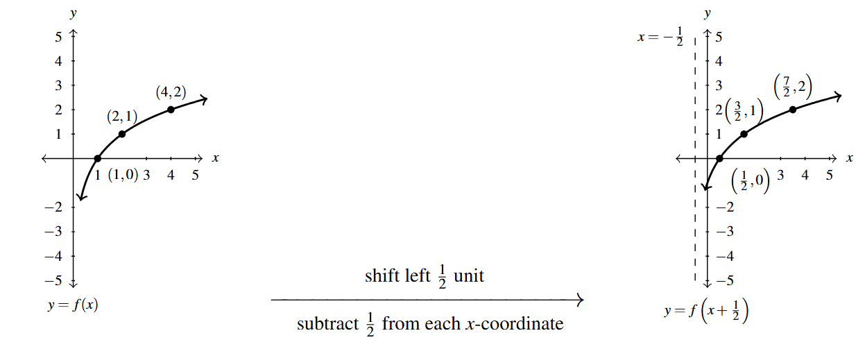
To write [latex]g(x)[/latex] in terms of [latex]f(x)[/latex], we note that based on points which are labeled, it appears as if the graph of [latex]g[/latex] can be obtained from the graph of [latex]f[/latex] by shifting the graph of [latex]f[/latex] to the right [latex]0.5[/latex] units and down 1 unit.
Per Theorems 1.8 and 1.7, [latex]g(x)[/latex] must take the form [latex]g(x) = f(x-h)+k[/latex]. Because the horizontal shift is to the right [latex]0.5[/latex] units, [latex]h = 0.5[/latex] and the vertical shift is down 1 unit, implies [latex]k = -1[/latex].
Hence, we get [latex]g(x) = f(x-0.5)-1[/latex].
We can check our answer by working through both transformations, in sequence, as in the previous example.
To write [latex]f(x)[/latex] in terms of [latex]g(x)[/latex], we need to reverse the process – that is, we need to shift the graph of [latex]g[/latex] left one half of a unit and up one unit. Theorems 1.8 and 1.7 suggest the formula [latex]f(x) = g(x+0.5)+1[/latex].
We leave it to the reader to check.
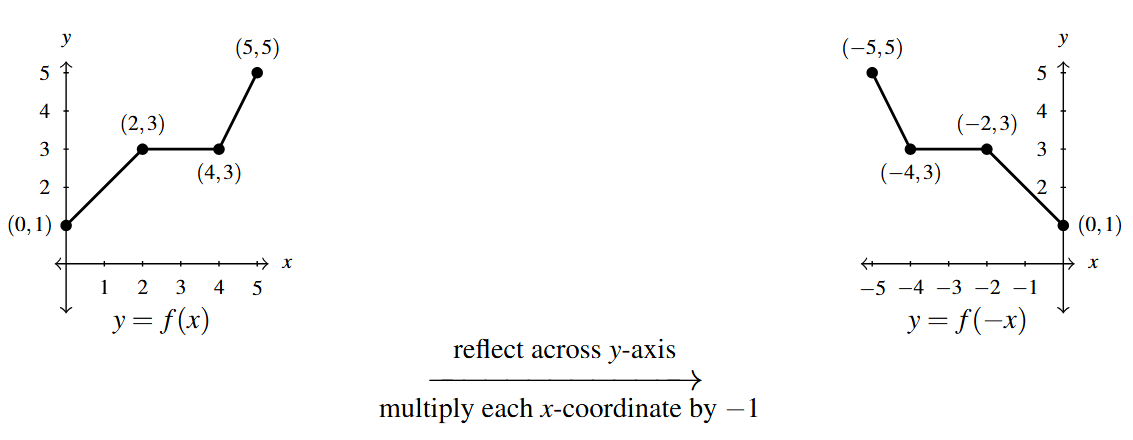
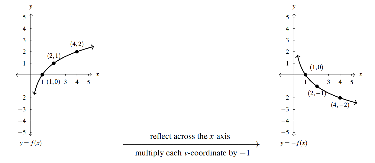
1.6.2 Reflections About the Coordinate Axes
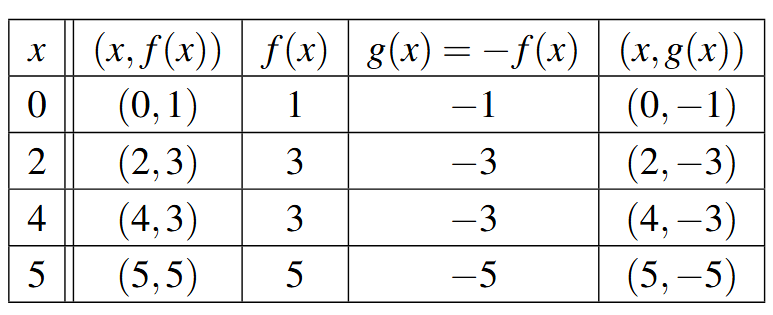
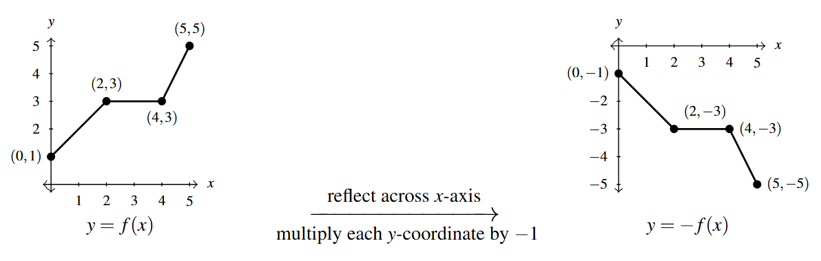
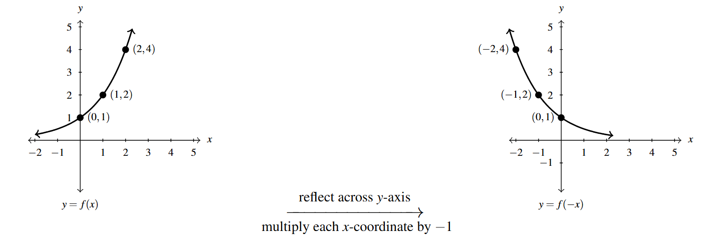
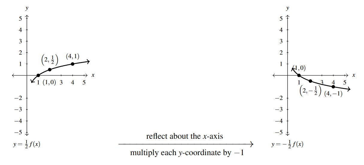
We now turn our attention to reflections. We know from Section 1.1 that to reflect a point [latex](x,y)[/latex] across the [latex]x[/latex]-axis, we replace [latex]y[/latex] with [latex]-y[/latex]. If [latex](x,y)[/latex] is on the graph of [latex]f[/latex], then [latex]y=f(x)[/latex], so replacing [latex]y[/latex] with [latex]-y[/latex] is the same as replacing [latex]f(x)[/latex] with [latex]-f(x)[/latex]. Hence, the graph of [latex]y=-f(x)[/latex] is the graph of [latex]f[/latex] reflected across the [latex]x[/latex]-axis. Similarly, the graph of [latex]y=f(-x)[/latex] is the graph of [latex]y = f(x)[/latex] reflected across the [latex]y[/latex]-axis.
Suppose [latex]f[/latex] is a function.
To graph [latex]F(x)=-f(x)[/latex], multiply each of the [latex]y[/latex]-coordinates of the points on the graph of [latex]y=f(x)[/latex] by [latex]-1[/latex].
NOTE: This results in a reflection across the [latex]x[/latex]-axis.
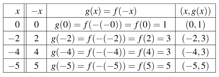
To graph [latex]F(x)=f(-x)[/latex], multiply each of the [latex]x[/latex]-coordinates of the points on the graph of [latex]y=f(x)[/latex] by [latex]-1[/latex].
NOTE: This results in a reflection across the [latex]y[/latex]-axis.
The proof of Theorem 1.9 follows in much the same way as the proofs of Theorems 1.7 and 1.8. If [latex]c[/latex] is an element of the domain of [latex]f[/latex] and [latex]F(x) = -f(x)[/latex], then the point [latex](c, f(c))[/latex] corresponds to the point [latex](c, F(c)) = (c,-f(c))[/latex]. Comparing the corresponding points [latex](c, f(c))[/latex] and [latex](c, -f(c))[/latex], we see they only difference is the [latex]y[/latex]-coordinates are the exact opposite – indicating they are mirror-images across the [latex]x[/latex]-axis. Similarly, if [latex]c[/latex] is an element in the domain of [latex]f[/latex], then [latex]c[/latex] corresponds to the element [latex]-c[/latex] in the domain of [latex]F(x) = f(-x)[/latex] because [latex]F(-c) = f(-(-c)) = f(c)[/latex]. Hence, the corresponding points here are [latex](c, f(c))[/latex] and [latex](-c, F(-c)) = (-c, f(c))[/latex]. Comparing [latex](c, f(c))[/latex] with [latex](-c, f(c))[/latex], we see they are reflections about the [latex]y[/latex]-axis.
Using the language of inputs and outputs, Theorem 1.9 says that multiplying the outputs from a function by [latex]-1[/latex] reflects its graph across the horizontal axis, while multiplying the inputs to a function by [latex]-1[/latex] reflects the graph across the vertical axis.
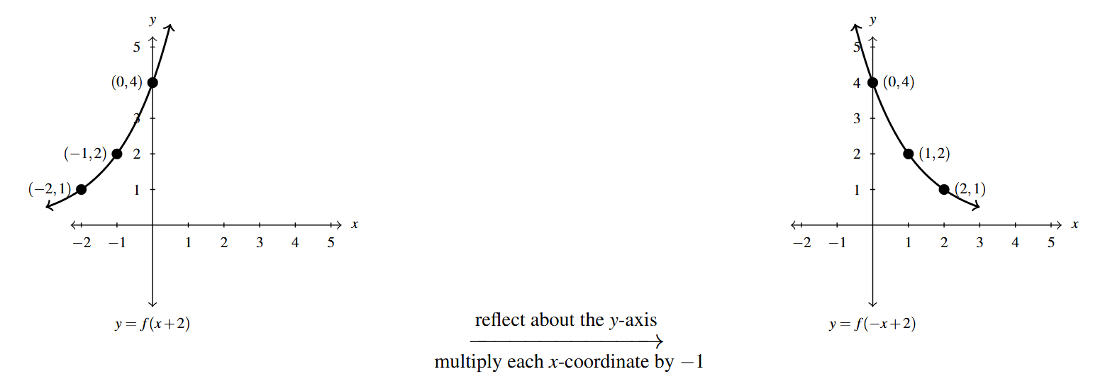
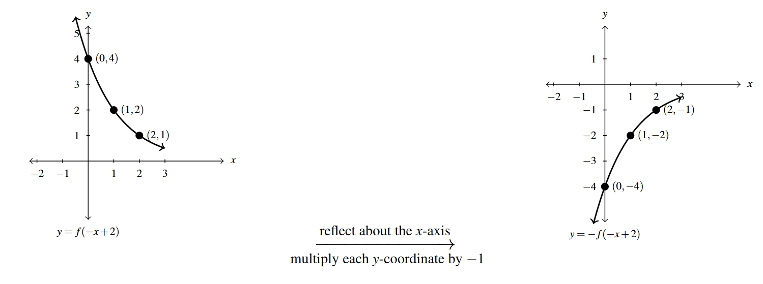
Applying Theorem 1.9 to the graph of [latex]y=f(x)[/latex] given at the beginning of the section, we can graph [latex]y=-f(x)[/latex] by reflecting the graph of [latex]f[/latex] about the [latex]x[/latex]-axis.
By reflecting the graph of [latex]f[/latex] across the [latex]y[/latex]-axis, we obtain the graph of [latex]y=f(-x)[/latex].
Example 1.6.2
Example 1.6.2.1a
Use Theorems 1.7, 1.8, and 1.9 to answer the questions below. Check your answers using a graphing utility where appropriate.
Suppose [latex](2,-5)[/latex] is on the graph of [latex]y = f(x)[/latex]. Find a point on the graph of:
[latex]y = f(-x)[/latex]
Solution:
Suppose [latex](2,-5)[/latex] is on the graph of [latex]y = f(x)[/latex]. Find a point on the graph of [latex]y=f(-x)[/latex].
To find a point on the graph of [latex]y=f(-x)[/latex], Theorem 1.9 tells us to multiply the [latex]x[/latex]-coordinate of the point on the graph of [latex]y=f(x)[/latex] by [latex]-1[/latex]: \[((-1)2, -5) = (-2,-5)\]
To check, given [latex](2,-5)[/latex] is on the graph of [latex]f[/latex], we know [latex]f(2) = -5[/latex]. Hence, when we substitute [latex]x=-2[/latex] into [latex]y = f(-x)[/latex], we get [latex]y = f(-(-2)) = f(2) = -5[/latex], proving [latex](-2,-5)[/latex] is on the graph of [latex]y=f(-x)[/latex].
Example 1.6.2.1b
Use Theorems 1.7, 1.8, and 1.9 to answer the questions below. Check your answers using a graphing utility where appropriate.
Suppose [latex](2,-5)[/latex] is on the graph of [latex]y = f(x)[/latex]. Find a point on the graph of:
[latex]y = -f(x+2)[/latex]
Solution:
Suppose [latex](2,-5)[/latex] is on the graph of [latex]y = f(x)[/latex]. Find a point on the graph of [latex]y=-f(x+2)[/latex].
To find a point on the graph of [latex]y = -f(x+2)[/latex], we first note we have two transformations at work here, so we work our way from the inside out and build [latex]f(x)[/latex] to [latex]-f(x+2)[/latex].
First, we find a point on the graph of [latex]y=f(x+2)[/latex]. Writing [latex]f(x+2) = f(x-(-2))[/latex], we apply Theorem 1.8 with [latex]h=-2[/latex] and add [latex]-2[/latex] to (or subtract 2 from) the [latex]x[/latex]-coordinate of the point we know is on [latex]y=f(x)[/latex]: [latex](2-2,-5) = (0,-5)[/latex].
Next, we apply Theorem 1.9 to the graph of [latex]y=f(x+2)[/latex] to get a point on the graph of [latex]y=-f(x+2)[/latex] by multiplying the [latex]y[/latex]-coordinate of [latex](0,-5)[/latex] by [latex]-1[/latex]: \[(0, (-1)(-5)) = (0,5)\]
To check, recall [latex]f(2)=-5[/latex], so that when we substitute [latex]x=0[/latex] into the equation [latex]y = -f(x+2)[/latex], we get [latex]y=-f(0+2) = -f(2) = -(-5)=5[/latex], as required.
Example 1.6.2.1c
Use Theorems 1.7, 1.8, and 1.9 to answer the questions below. Check your answers using a graphing utility where appropriate.
Suppose [latex](2,-5)[/latex] is on the graph of [latex]y = f(x)[/latex]. Find a point on the graph of:
[latex]f(8-x)[/latex]
Solution:
Suppose [latex](2,-5)[/latex] is on the graph of [latex]y = f(x)[/latex]. Find a point on the graph of [latex]y=f(8-x)[/latex].
Rewriting [latex]f(8-x) = f(-x+8)[/latex] we see we have two transformations at play here: a reflection across the [latex]y[/latex]-axis and a horizontal shift. Both of these transformations affect the [latex]x[/latex]-coordinates of the graph, thus the question becomes which transformation to address first. To help us with this decision, we attack the problem algebraically.
Recall that [latex](2,-5)[/latex] is on the graph of [latex]f[/latex], so we know [latex]f(2) = -5[/latex]. Hence, to get a point on the graph of [latex]y = f(-x+8)[/latex], we need to match up the arguments of [latex]f(-x+8)[/latex] and [latex]f(2)[/latex]: [latex]-x+8 = 2[/latex].
To solve this equation, we first subtract [latex]8[/latex] from both sides to get [latex]-x = -6[/latex]. Geometrically, subtracting [latex]8[/latex] from the [latex]x[/latex]-coordinate of [latex](2,-5)[/latex], shifts the point [latex](2,-5)[/latex] left [latex]8[/latex] units to get the point [latex](-6,-5)[/latex].
Next, we multiply both sides of the equation [latex]-x = -6[/latex] by [latex]-1[/latex] to get [latex]x = 6[/latex]. Geometrically, multiplying the [latex]x[/latex]-coordinate of [latex](-6,-5)[/latex] by [latex]-1[/latex] reflects the point [latex](-6,-5)[/latex] across the [latex]y[/latex]-axis to [latex](6,-5)[/latex].
To check we substitute [latex]x=6[/latex] into [latex]y = f(-x+8)[/latex], and obtain [latex]y = f(-6+8) = f(2) = -5[/latex].
Even though we have found our answer, we re-examine this process from a build perspective. We began with a point on the graph of [latex]y=f(x)[/latex] and first shifted the graph to the left [latex]8[/latex] units. Per Theorem 1.8, this point is on the graph of [latex]y=f(x+8)[/latex].
Next we took a point on the graph of [latex]y=f(x+8)[/latex] and reflected it about the [latex]y[/latex]-axis. Per Theorem 1.9, this put the point on the graph of [latex]y=f(-x+8)[/latex].
In general, when faced with graphing functions in which there is both a horizontal shift and a reflection about the [latex]y[/latex]-axis, we’ll deal with the shift first.
Example 1.6.2.2
Use Theorems 1.7, 1.8, and 1.9 to answer the questions below. Check your answers using a graphing utility where appropriate.
Write a formula for a function [latex]H(s)[/latex] whose graph is the same as [latex]t=h(s) = s^3-s^2[/latex] but is reflected across the [latex]t[/latex]-axis.
Solution:
Write a formula for a function [latex]H(s)[/latex] whose graph is the same as [latex]t=h(s) = s^3-s^2[/latex] but is reflected across the [latex]t[/latex]-axis.
In this example, the independent variable is [latex]s[/latex] and the dependent variable is [latex]t[/latex]. We are asked to reflect the graph of [latex]h[/latex] (in red) about the [latex]t[/latex]-axis, which in this case is the vertical axis.
Hence, [latex]H(s) = h(-s) = (-s)^3-(-s)^2 = -s^3-s^2[/latex] (in blue).
Our confirmation is below.
Example 1.6.2.3
Use Theorems 1.7, 1.8, and 1.9 to answer the questions below. Check your answers using a graphing utility where appropriate.
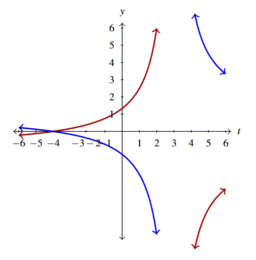
Predict how the graph of [latex]G(t) = \dfrac{t+4}{t-3}[/latex] relates to the graph of [latex]g(t) =\dfrac{t+4}{3-t}[/latex].
Solution:
Predict how the graph of [latex]G(t) = \dfrac{t+4}{t-3}[/latex] relates to the graph of [latex]g(t) =\dfrac{t+4}{3-t}[/latex] .
Comparing the formulas for [latex]G(t) = \dfrac{t+4}{t-3}[/latex] and [latex]g(t) =\dfrac{t+4}{3-t}[/latex], we have the same numerators, but in the denominator, we have [latex](t-3) = -(3-t)[/latex]:\[ \begin{array}{rcl} G(t) &=& \dfrac{t+4}{t-3}\\ &=& \dfrac{t+4}{-(3-t)}\\ &=& – \dfrac{t+4}{3-t}\\ &=& -g(t). \end{array}\]
Hence, the graph of [latex]y=G(t)[/latex] (in blue) should be the graph of [latex]y=g(t)[/latex] (in red) reflected across the [latex]t[/latex]-axis.
Example 1.6.2.4a
Use Theorems 1.7, 1.8, and 1.9 to answer the questions below. Check your answers using a graphing utility where appropriate.
Below is the graph of [latex]y = f(x)[/latex].
Use it to sketch the graph of
[latex]F(x) = f(-x)+1[/latex]
Solution:
Sketch the graph of [latex]F(x) = f(-x)+1[/latex].
We have two transformations indicated with the formula [latex]F(x) = f(-x)+1[/latex]: a reflection across the [latex]y[/latex]-axis and a vertical shift.
Working from the inside out, we first tackle the reflection. Per Theorem 1.9, to obtain the graph of [latex]y=f(-x)[/latex] from [latex]y=f(x)[/latex], we multiply each of the [latex]x[/latex]-coordinates of each of the points on the graph of [latex]y=f(x)[/latex] by [latex](-1)[/latex].
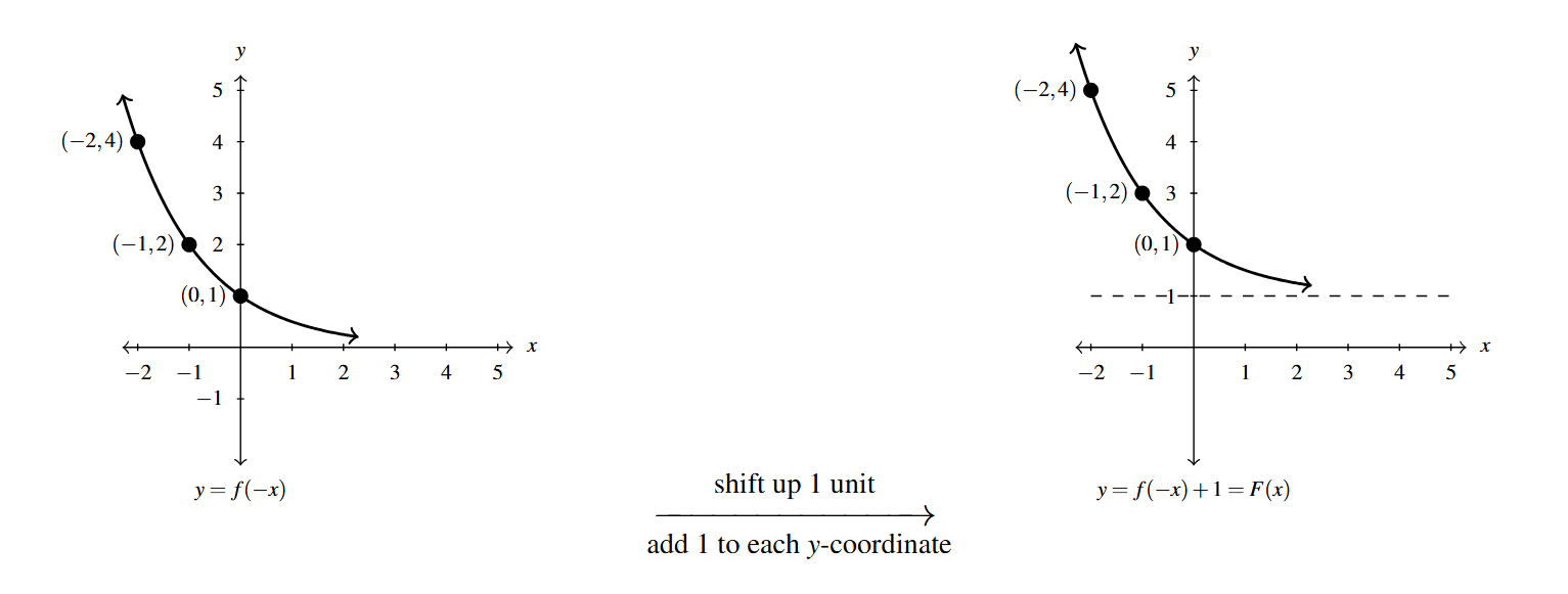
Next, we use Theorem 1.7 to obtain the graph of [latex]y =f(-x)+1[/latex] from the graph of [latex]y = f(-x)[/latex] by adding 1 to each of the [latex]y[/latex]-coordinates of each of the points on the graph of [latex]y = f(-x)[/latex]. This shifts the graph of [latex]y=f(-x)[/latex] up one unit. Note, the horizontal asymptote [latex]y=0[/latex] is also shifted up 1 unit to [latex]y=1[/latex].
To check our answer, we begin with the point [latex](0,2)[/latex]. Substituting [latex]x=0[/latex] into [latex]y=f(-x)+1[/latex], we get [latex]y=f(-0)+1 = f(0)+1[/latex]. Given the point [latex](0,1)[/latex] is on the graph of [latex]f[/latex], we know [latex]f(0) = 1[/latex]. Hence, [latex]y = f(0)+1= 1+1=2[/latex], so [latex](0,2)[/latex] is, indeed, on the graph of [latex]y=f(-x)+1[/latex]. We leave it to the reader to check the remaining points.
Example 1.6.2.4b
Use Theorems 1.7, 1.8, and 1.9 to answer the questions below. Check your answers using a graphing utility where appropriate.
Below is the graph of [latex]y = f(x)[/latex].
[latex]F(x)= 1 - f(2-x)[/latex]
Solution:
Sketch the graph of [latex]F(x) = 1-f(2-x)[/latex].
In order to graph [latex]F(x)= 1 - f(2-x)[/latex], we first rewrite as [latex]F(x) = -f(-x+2)+1[/latex] and note there are four modifications to the formula [latex]f(x)[/latex] indicated here.
Working from the inside out, we see we have a reflection about the [latex]y[/latex]-axis indicated as well as a horizontal shift. From our work above, we know we first handle the shift: that is, we apply Theorem 1.8 to graph [latex]y=f(x+2) = f(x-(-2))[/latex] by adding [latex]-2[/latex] to (subtracting 2 from) the [latex]x[/latex]-coordinates of the points on the graph of [latex]y=f(x)[/latex].
Next, we use Theorem 1.9 to graph [latex]y=f(-x+2)[/latex] starting with the graph of [latex]y = f(x+2)[/latex] by multiplying each of the [latex]x[/latex]-coordinates of the points of the graph of [latex]y=f(x+2)[/latex] by [latex]-1[/latex]. This reflects the graph of [latex]f(x+2)[/latex] about the [latex]y[/latex]-axis.
We have the graph of [latex]y=f(-x+2)[/latex] and need to build towards the graph of [latex]y=-f(-x+2)+1[/latex]. The transformations that remain are a reflection about the [latex]x[/latex]-axis and a vertical shift. The question is which to do first.
Once again, we can think algebraically about the problem. We know the point [latex](0,1)[/latex] is on the graph of [latex]f[/latex] which means [latex]f(0) = 1[/latex]. This point corresponds to the point [latex](2,1)[/latex] on the graph of [latex]f(-x+2)[/latex]. Indeed, when we substitute [latex]x=2[/latex] into [latex]y=f(-x+2)[/latex], we get [latex]y = f(-2+2) = f(0) =1[/latex].
If we substitute [latex]x=2[/latex] into the formula [latex]y=-f(-x+2)+1[/latex], we get [latex]y=-f(-2+2)+1 = -f(0)+1 = -1(1)+1 = 0[/latex]. That is, we first multiply the [latex]y[/latex]-coordinate of [latex](2,1)[/latex] by [latex]-1[/latex] and then add 1. This suggests we take care of the reflection about the [latex]x[/latex]-axis first, then the vertical shift.
We proceed below to obtain the graph of [latex]y=-f(-x+2)[/latex] from [latex]y=f(-x+2)[/latex] by multiplying each of the [latex]y[/latex]-coordinates on the graph of [latex]y=f(-x+2)[/latex] by [latex]-1[/latex]. Note the horizontal asymptote remains unchanged: [latex]y=(-1)(0) = 0[/latex].
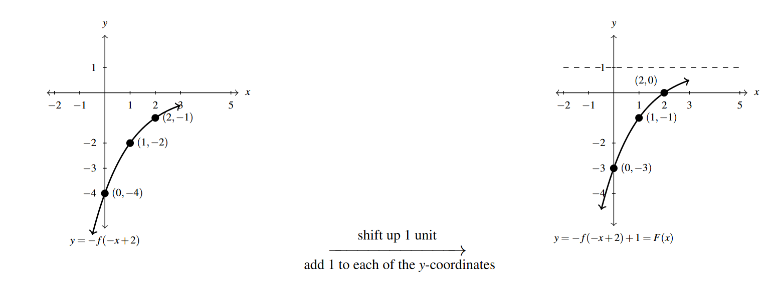
Finally, we take care of the vertical shift. Per Theorem 1.7, we graph [latex]y=-f(-x+2)+1[/latex] by adding 1 to the [latex]y[/latex]-coordinates of each of the points on the graph of [latex]y=-f(-x+2)[/latex]. This moves the graph up one unit, including the horizontal asymptote: [latex]y=0+1 = 1[/latex].
To check, we begin with the point [latex](2,0)[/latex]. Substituting [latex]x=2[/latex] into [latex]y=1 - f(2-x)[/latex], we obtain [latex]y = 1-f(2-2) = 1-f(0)[/latex]. Given [latex](0,1)[/latex] is on the graph of [latex]f[/latex], we know [latex]f(0) = 1[/latex]. This means [latex]y = 1-f(2-2) = 1-f(0)= 1-1 = 0[/latex]. This proves [latex](2,0)[/latex] is on the graph of [latex]y=1 - f(2-x)[/latex], and we recommend the reader check the remaining points.
Example 1.6.2.5
Use Theorems 1.7, 1.8, and 1.9 to answer the questions below. Check your answers using a graphing utility where appropriate.
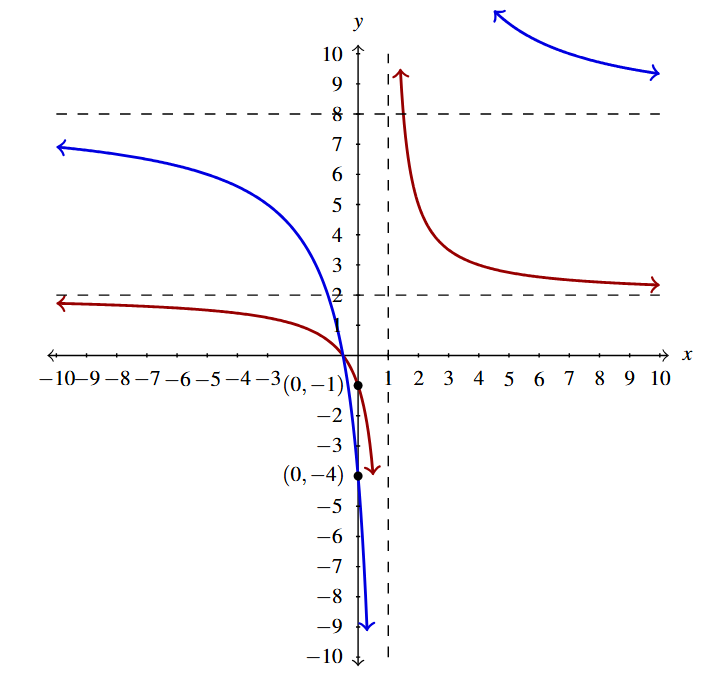
Below is the graph of [latex]y = g(x)[/latex]. Write [latex]g(x)[/latex] in terms of [latex]f(x)[/latex] from part 4 and vice-versa.
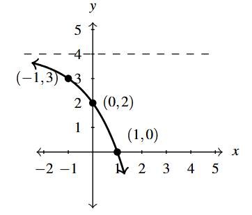
NOTE: The [latex]x[/latex]-axis, [latex]y=0[/latex], is a horizontal asymptote to the graph of [latex]y = f(x)[/latex] and the line [latex]y=4[/latex] is a horizontal asymptote to the graph of [latex]y = g(x)[/latex].
Solution:
Write [latex]g(x)[/latex] in terms of [latex]f(x)[/latex] and visa-versa.
With the transformations at our disposal, our task amounts to finding values of [latex]h[/latex] and [latex]k[/latex] and choosing between signs [latex]\pm[/latex] so that [latex]g(x) = \pm f( \pm x - h) + k[/latex].
Based on the horizontal asymptote, [latex]y=4[/latex], we choose [latex]k=4[/latex]. Note, however, in the graph of [latex]y=f(x)+4[/latex], the entire graph is above the line [latex]y=4[/latex]. Due to the fact that the graph of [latex]g[/latex] approaches the asymptote from below, we know [latex]y=-f(\pm x-h)+4[/latex].
Hence, two of transformations applied to the graph of [latex]f[/latex] are a reflection across the [latex]x[/latex]-axis followed by a shift up [latex]4[/latex] units. This means the point [latex](0,1)[/latex] on the graph of [latex]f[/latex] must correspond to the point [latex](-1,3)[/latex] on the graph of [latex]g[/latex], as these are the points closest to their respective asymptotes.
Likewise, the points [latex](1,2)[/latex] and [latex](2,4)[/latex] on the graph of [latex]f[/latex] must correspond to [latex](0,2)[/latex] and [latex](1,0)[/latex], respectively, on the graph of [latex]g[/latex]. Looking at the [latex]x[/latex]-coordinates only, we have [latex]x=0[/latex] moves to [latex]x=-1[/latex], [latex]x=1[/latex] moves to [latex]x=0[/latex], and [latex]x=2[/latex] moves to [latex]x=1[/latex]. Hence, the net effect on the [latex]x[/latex]-values is a shift left 1 unit. Hence, we guess the formula for [latex]g(x)[/latex] to be [latex]g(x) = -f(x+1)+4[/latex].
We can readily check by going through the transformations: first, shift left 1 unit; next, reflect across the [latex]x[/latex]-axis; finally, shift up [latex]4[/latex]. We leave it to the reader to verify that tracking each of the points on the graph of [latex]f[/latex] along with the horizontal asymptote through this sequence of transformations results in the graph of [latex]g[/latex].
One way to recover the graph of [latex]f[/latex] from the graph of [latex]g[/latex] is to reverse the process by which we obtained [latex]g[/latex] from [latex]f[/latex]. The challenge here comes from the fact that two different operations were done which affected the [latex]y[/latex]-values: reflection and shifting – and the order in which these are done matters.
To motivate our methodology, let’s consider a more down-to-earth example like putting on socks and then putting on shoes. Unless we’re very talented, to reverse this process, we take off the shoes first, then the socks – that is, we undo each step in the reverse order.[1] In the same way, when we think about reversing the steps transforming the graph of [latex]f[/latex] to the graph of [latex]g[/latex], we need to undo each transformation in the opposite order.
To review, we obtained the graph of [latex]g[/latex] from the graph of [latex]f[/latex] by first shifting the graph to the left 1 unit, then reflecting the graph about the [latex]x[/latex]-axis, then, finally, shifting the graph up [latex]4[/latex] units. Hence, we first undo the vertical shift. Instead of shifting the graph up four units, we shift the graph down four units. This takes the graph of [latex]y = g(x)[/latex] to [latex]y = g(x)-4[/latex].
Next, we have to undo the refection across the [latex]x[/latex]-axis. Thinking at the level of points, to recover the point [latex](a,b)[/latex] from its reflection across the [latex]x[/latex]-axis, [latex](a,-b)[/latex], we simply reflect across the [latex]x[/latex]-axis again: [latex](a,-(-b)) = (a,b)[/latex]. Per Theorem 1.9, this takes the graph the graph of [latex]y = g(x)-4[/latex] to the graph of [latex]y = -[g(x)-4] = -g(x) + 4[/latex].[2]
Last, to undo moving the graph to the left 1 unit, we move the graph of [latex]y=-g(x)+4[/latex] to the right 1 unit. Per Theorem 1.8, we accomplish this by graphing [latex]y = -g(x-1)+4[/latex]. We leave it to the reader to start with the graph of [latex]y=g(x)[/latex] and graph [latex]y = -g(x-1)+4[/latex] and show it matches the graph of [latex]y=f(x)[/latex].
Some remarks about Example 1.6.2 are in order. In number 1c above, to find a point on the graph of [latex]y=f(-x+8)[/latex], we took the given [latex]x[/latex]-coordinate on our starting graph, 2, and subtracted [latex]8[/latex] first then multiplied by [latex]-1[/latex]. If this seems somehow backwards it should.
When evaluating the expression [latex]-x+8[/latex], the order of operations mandates we multiply by [latex]-1[/latex] first then add [latex]8[/latex]. Here, however, we weren’t evaluating an expression – we were solving an equation: [latex]-x+8 = 2[/latex], which meant we did the exact opposite steps in the opposite order.\footnote{Note that dividing by [latex]-1[/latex] is the same as multiplying by [latex]-1[/latex], so to keep with the opposite steps in opposite order theme, we could more precisely say we subtracted [latex]8[/latex] and divided by [latex]-1[/latex].} This exemplifies a larger theme with transformations: when adjusting inputs, the resulting points on the graph are obtained by applying the opposite operations indicated by the formula in the opposite order of operations.
On the other hand, when it came to multiple transformations involving the [latex]y[/latex]-coordinates, we followed the order of operations. As in 4b above, when it came to applying a reflection about the [latex]x[/latex]-axis and a vertical shift, we applied the reflection first, then the shift. This is because instead of solving an equation to find the new [latex]y[/latex]-coordinates, we were simplifying an expression. Again, this is an example of a much larger theme: when adjusting outputs, the resulting points on the graph are obtained by applying the stated operations in the usual order.
Last but not least, in number 5, to find [latex]f[/latex] in terms of [latex]g[/latex], we reversed the steps used to transform [latex]f[/latex] into [latex]g[/latex]. Another tact is to approach the problem in the same way we approached transforming [latex]f[/latex] into [latex]g[/latex]: namely, starting with the graph of [latex]g[/latex], determine values [latex]h[/latex] and [latex]k[/latex] and signs [latex]\pm[/latex] so that [latex]f(x) = \pm g(\pm x - h) + k[/latex]. We leave this to the reader.
1.6.3 Scalings
We now turn our attention to our last class of transformations: scalings. A thorough discussion of scalings can get complicated because they are not as straight-forward as the previous transformations. A quick review of what we’ve covered so far, namely vertical shifts, horizontal shifts and reflections, will show you why those transformations are known as rigid transformations.
Simply put, rigid transformations preserve the distances between points on the graph – only their position and orientation in the plane change.[3] If, however, we wanted to make a new graph twice as tall as a given graph, or one-third as wide, we would be affecting the distance between points. These sorts of transformations are hence called non-rigid. As always, we motivate the general theory with an example.
Suppose we wish to graph the function [latex]g(x) =2 f(x)[/latex] where [latex]f(x)[/latex] is the function whose graph is given at the beginning of the section. From its graph, we can build a table of values for [latex]g[/latex] as before.
Graphing, we get
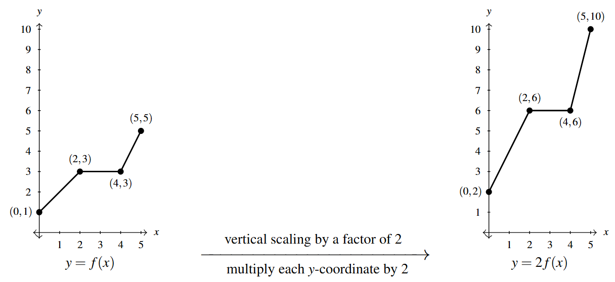
In general, if [latex](a,b)[/latex] is on the graph of [latex]f[/latex], then [latex]f(a) = b[/latex] so that [latex]g(a) = 2 f(a) = 2b[/latex] puts [latex](a,2b)[/latex] on the graph of [latex]g[/latex]. In other words, to obtain the graph of [latex]g[/latex], we multiply all of the [latex]y[/latex]-coordinates of the points on the graph of [latex]f[/latex] by 2. Multiplying all of the [latex]y[/latex]-coordinates of all of the points on the graph of [latex]f[/latex] by 2 causes what is known as a vertical scaling[4] by a factor of 2.
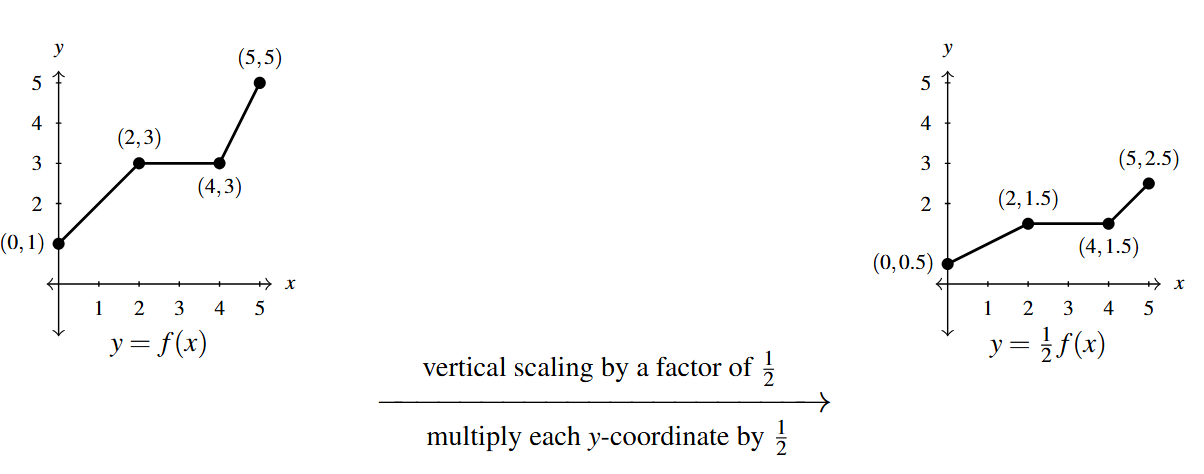
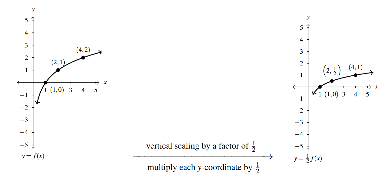
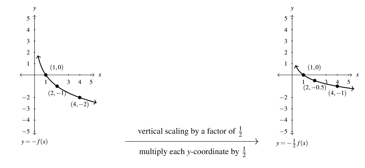
If we wish to graph [latex]y = \dfrac{1}{2} f(x)[/latex], we multiply the all of the [latex]y[/latex]-coordinates of the points on the graph of [latex]f[/latex] by [latex]\dfrac{1}{2}[/latex]. This creates a vertical scaling[5] by a factor of [latex]\dfrac{1}{2}[/latex] as seen below.
These results are generalized in the following theorem.
Suppose [latex]f[/latex] is a function and [latex]a>0[/latex] is a real number.
To graph [latex]F(x) = a\,f(x)[/latex], multiply each of the [latex]y[/latex]-coordinates of the points on the graph of [latex]y=f(x)[/latex] by [latex]a[/latex].
- If [latex]a > 1[/latex], we say the graph of [latex]f[/latex] has undergone a vertical stretch[6] by a factor of [latex]a[/latex].
- If [latex]0[/latex] < [latex]a[/latex] < [latex]1[/latex], we say the graph of [latex]f[/latex] has undergone a vertical shrink[7] by a factor of [latex]\dfrac{1}{a}[/latex].
The proof of Theorem 1.10 mimics the proofs of Theorems 1.7 and 1.9. If [latex]c[/latex] is in the domain of [latex]f[/latex], then [latex](c, f(c))[/latex] is on the graph of [latex]f[/latex] and the corresponding point on the graph of [latex]F(x)=a \, f(x)[/latex] is [latex](c, F(c)) = (c, a \, f(c))[/latex]. Comparing the points [latex](c, f(c))[/latex] and [latex](c, a \, f(c))[/latex] proves the theorem.
A few remarks about Theorem 1.10 are in order. First, a note about the verbiage. To the authors, the words stretch, expansion, and dilation all indicate something getting bigger. Hence, stretched by a factor of 2 makes sense if we are scaling something by multiplying it by 2. Similarly, we believe words like shrink, compression and contraction all indicate something getting smaller, so if we scale something by a factor of [latex]\dfrac{1}{2}[/latex], we would say it shrinks by a factor of 2 – not shrinks by a factor of [latex]\dfrac{1}{2}[/latex]. This is why we have written the descriptions stretch by a factor of [latex]a[/latex] and shrink by a factor of [latex]\dfrac{1}{a}[/latex] in the statement of the theorem.
Second, in terms of inputs and outputs, Theorem 1.10 says multiplying the outputs from a function by positive number [latex]a[/latex] causes the graph to be vertically scaled by a factor of [latex]a[/latex]. It is natural to ask what would happen if we multiply the inputs of a function by a positive number. This leads us to our last transformation of the section.
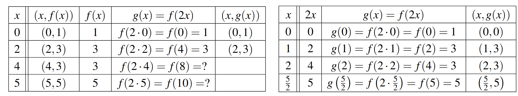
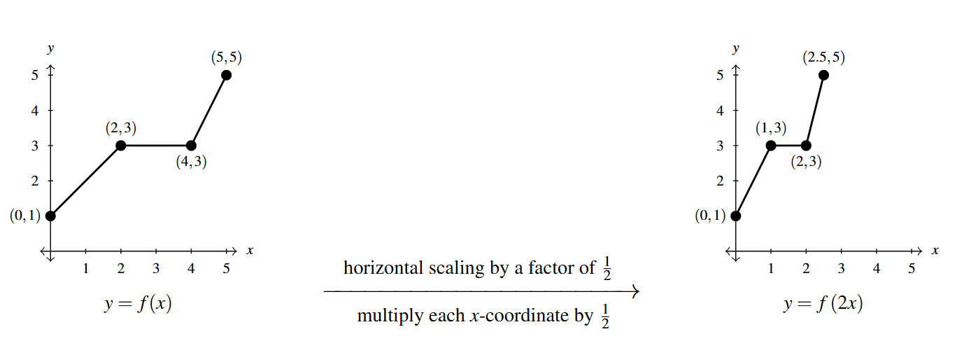
Referring to the graph of [latex]f[/latex] given at the beginning of this section, suppose we want to graph [latex]g(x) = f(2x)[/latex]. In other words, we are looking to see what effect multiplying the inputs to [latex]f[/latex] by 2 has on its graph. If we attempt to build a table directly, we quickly run into the same problem we had in our discussion leading up to Theorem 1.8, as seen in the table on the left below.
We solve this problem in the same way we solved this problem before. For example, if we want to determine the point on [latex]g[/latex] which corresponds to the point [latex](2,3)[/latex] on the graph of [latex]f[/latex], we set [latex]2x =2[/latex] so that [latex]x=1[/latex]. Substituting [latex]x=1[/latex] into [latex]g(x)[/latex], we obtain [latex]g(1) = f(2 \cdot 1) = f(2) = 3[/latex], so that [latex](1,3)[/latex] is on the graph of [latex]g[/latex]. Continuing in this fashion, we obtain the table on the lower right.
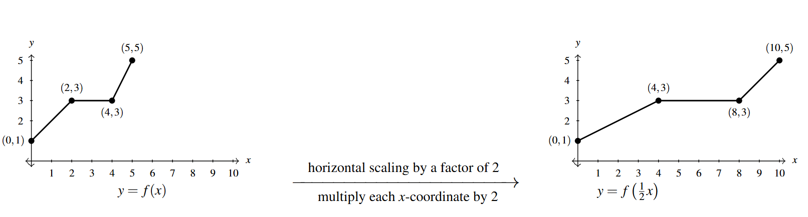
If, on the other hand, we wish to graph [latex]y = f\left( \dfrac{1}{2} x\right)[/latex], we end up multiplying the [latex]x[/latex]-coordinates of the points on the graph of [latex]f[/latex] by 2 which results in a horizontal scaling[9] by a factor of 2, as demonstrated below.
We have the following theorem.
Suppose [latex]f[/latex] is a function and [latex]b>0[/latex] is a real number.
To graph [latex]F(x) = f(bx)[/latex], divide each of the [latex]x[/latex]-coordinates of the points on the graph of [latex]y=f(x)[/latex] by [latex]b[/latex].
- If [latex]0[/latex] < [latex]b[/latex] < [latex]1[/latex], we say the graph of [latex]f[/latex] has undergone a horizontal stretch[10] by a factor of [latex]\dfrac{1}{b}[/latex].
- If [latex]b > 1[/latex], we say the graph of [latex]f[/latex] has undergone a horizontal shrink[11] by a factor of [latex]b[/latex].
The proof of Theorem 1.11 follows closely the spirit of the proof of Theorems 1.8 and 1.9. If [latex]c[/latex] is an element of the domain of [latex]f[/latex], then the number [latex]\dfrac{c}{b}[/latex] corresponds to a domain element of [latex]F(x)= f(bx)[/latex] due to the fact that [latex]F\left(\dfrac{c}{b} \right) = f\left( b \cdot \dfrac{c}{b} \right) = f(c)[/latex]. Hence, there is a correspondence between the point [latex](c, f(c))[/latex] on the graph of [latex]f[/latex] and the point [latex]\left( \dfrac{c}{b}, F\left(\dfrac{c}{b}\right) \right)= \left( \dfrac{c}{b}, f(c) \right)[/latex] on the graph of [latex]F[/latex]. We can obtain [latex]\left( \dfrac{c}{b}, f(c) \right)[/latex] by dividing the [latex]x[/latex]-coordinate of [latex](c, f(c))[/latex] by [latex]b[/latex] and the result follows.
Theorem 1.11 tells us that if we multiply the input to a function by [latex]b[/latex], the resulting graph is scaled horizontally by a factor of [latex]\dfrac{1}{b}[/latex]. The next example explores how vertical and horizontal scalings sometimes interact with each other and with the other transformations introduced in this section.
Example 1.6.3
Example 1.6.3.1a
Use Theorems 1.7, 1.8, 1.9, 1.10, and 1.11 to answer the questions below. Check your answers using a graphing utility where appropriate.
Suppose [latex](-1,4)[/latex] is on the graph of [latex]y = f(x)[/latex]. Find a point on the graph of:
[latex]y = 3f(x-2)[/latex]
Solution:
Suppose [latex](-1,4)[/latex] is on the graph of [latex]y = f(x)[/latex]. Find a point on the graph of [latex]y=3f(x-2)[/latex].
As we examine the formula [latex]y = 3f(x-2)[/latex], we note two modifications from [latex]y=f(x)[/latex]. Building from the inside out, we start with obtaining a point on the graph of [latex]y=f(x-2)[/latex].
Per Theorem 1.8, this shifts all of the points on the graph of [latex]y=f(x)[/latex] right 2 units. Hence, the point [latex](-1,4)[/latex] on the graph of [latex]y=f(x)[/latex] moves to the point [latex](-1+2, 4) = (1,4)[/latex] on the graph of [latex]y=f(x-2)[/latex].
To get a point on the graph of [latex]y = 3f(x-2) = a f(x-2)[/latex], we apply Theorem 1.10 with [latex]a=3[/latex] to the point [latex](1,4)[/latex] on the graph of [latex]y=f(x-2)[/latex] to get the point [latex](1,3(4)) = (1,12)[/latex] on the graph of [latex]y=3f(x-2)[/latex].
To check, we note that given [latex](-1,4)[/latex] is on the graph of [latex]y=f(x)[/latex], we know [latex]f(-1)=4[/latex]. Hence, when we substitute [latex]x=1[/latex] into the [latex]y=3f(x-2)[/latex], we get [latex]y=3f(1-2) = 3f(-1) = 3(4) = 12[/latex].
Example 1.6.3.1b
Use Theorems 1.7, 1.8, 1.9, 1.10, and 1.11 to answer the questions below. Check your answers using a graphing utility where appropriate.
Suppose [latex](-1,4)[/latex] is on the graph of [latex]y = f(x)[/latex]. Find a point on the graph of:
[latex]y = f\left(-\dfrac{1}{2} x \right)[/latex]
Solution:
Suppose [latex](-1,4)[/latex] is on the graph of [latex]y = f(x)[/latex]. Find a point on the graph of [latex]y = f \left( - \dfrac{1}{2} x \right)[/latex].
The formula [latex]y = f\left(-\dfrac{1}{2} x \right)[/latex] also indicates two transformations: a horizontal scaling, indicated by [latex]\dfrac{1}{2}[/latex] factor, as well as a reflection across the [latex]y[/latex]-axis. The question before us is which to do first.
If we return to algebra for inspiration, we know [latex]f(-1) = 4[/latex], so we match up the arguments of [latex]f\left(-\dfrac{1}{2} x \right)[/latex] and [latex]f(-1)[/latex] and get the equation [latex]-\dfrac{1}{2} x = -1[/latex]. We solve this equation by multiplying both sides by [latex]-2[/latex]: [latex]x = (-2)(-1) = 2[/latex]. That is, we take the original [latex]x[/latex]-value on the graph of [latex]y=f(x)[/latex] and multiply it by [latex]-2[/latex].
If we think of [latex]-2= (-1)(2)[/latex], then multiplying by the 2 in [latex](-1)(2)[/latex] produces a horizontal stretch by a factor of 2, while multiplying by the [latex]-1[/latex] reflects the point across the [latex]y[/latex]-axis.
Applying the horizontal stretch first, we use Theorem 1.11 and start with the point [latex](-1,4)[/latex] on the graph of [latex]y=f(x)[/latex] and multiply the [latex]x[/latex]-coordinate by 2 to obtain a point on the graph of [latex]y=f\left(\dfrac{1}{2} x\right)[/latex]: [latex](-1(2), 4) = (-2,4)[/latex].
Next, we take care of the reflection about the [latex]y[/latex]-axis, using Theorem 1.9. Starting with [latex](-2,4)[/latex] on the graph of [latex]y=f\left(\dfrac{1}{2} x \right)[/latex], we multiply the [latex]x[/latex]-coordinate by [latex]-1[/latex] to obtain a point on the graph of [latex]y = f\left(\dfrac{1}{2} (-x) \right) = f\left(-\dfrac{1}{2} x \right)[/latex]: [latex]((-1)(-2),4) = (2,4)[/latex].
To check, note when [latex]x=2[/latex] is substituted into [latex]y = f\left(-\dfrac{1}{2} x \right)[/latex], we get [latex]y = f\left(-\dfrac{1}{2} (2) \right) = f(-1) = 4[/latex].
Of course, we could have equally written the multiple [latex]-2 = (2)(-1)[/latex] and reversed these steps: doing the reflection first, then the horizontal scaling.
Proceeding this way, we start with the point [latex](-1,4)[/latex] on the graph of [latex]y=f(x)[/latex] and reflect across the [latex]y[/latex]-axis to obtain the point [latex]((-1)(-1), 4) = (1,4)[/latex] on the graph of [latex]y = f(-x)[/latex].
Next, we stretch the graph of [latex]y=f(-x)[/latex] by a factor of 2 by multiplying the [latex]x[/latex]-coordinates of the points on the graph by 2 and obtain [latex](2(1), 4) = (2,4)[/latex] on the graph of [latex]y=f\left(-\dfrac{1}{2} x\right)[/latex].
In general when it comes to reflections and scalings, whether horizontal or, as we’ll see soon, vertical, either order will produce the same results.
Example 1.6.3.1c
Use Theorems 1.7, 1.8, 1.9, 1.10, and 1.11 to answer the questions below. Check your answers using a graphing utility where appropriate.
Suppose [latex](-1,4)[/latex] is on the graph of [latex]y = f(x)[/latex]. Find a point on the graph of:
[latex]f(2x-3)+1[/latex]
Solution:
Suppose [latex](-1,4)[/latex] is on the graph of [latex]y = f(x)[/latex]. Find a point on the graph of [latex]y=f(2x-3)+1[/latex].
The formula [latex]f(2x-3)+1[/latex] indicates three transformations: a horizontal shift, a horizontal scaling, and a vertical shift. As usual, we appeal to algebra to give us guidance on which horizontal transformation to apply first.
Given [latex]f(-1) = 4[/latex], we set [latex]2x-3 = -1[/latex] and solve for [latex]x[/latex]. Our first step is to add 3 to both sides: [latex]2x=(-1)+3 =2[/latex]. Because we are adding 3 to the given [latex]x[/latex]-value [latex]-1[/latex], this corresponds to a shift to the right 3 units, so the point [latex](-1,4)[/latex] is moved to the point [latex](2,4)[/latex].
Next, to solve [latex]2x=2[/latex], we divide this new [latex]x[/latex]-coordinate 2 by 2 and get [latex]x = \dfrac{2}{2}=1[/latex] which corresponds to a horizontal compression by a factor of 2. This moves the point [latex](2,4)[/latex] to [latex](1,4)[/latex].
Hence, the algebra suggests we use Theorem 1.8 first and follow it up with Theorem 1.11. Starting with [latex](-1,4)[/latex] on the graph of [latex]y=f(x)[/latex], we shift to the right 3 units to obtain the point [latex](-1+3, 4) = (2,4)[/latex] on the graph of [latex]y=f(x-3)[/latex].
Next, we start with the point [latex](2,4)[/latex] on the graph of [latex]y=f(x-3)[/latex] and horizontally shrink the [latex]x[/latex]-axis by a factor of 2 to get the point [latex]\left(\dfrac{2}{2}, 4\right) = (1,4)[/latex] on the graph of [latex]y=f(2x-3)[/latex].
Last, but not least, we take care of the vertical shift using Theorem 1.7. Starting with the point [latex](1,4)[/latex] on the graph of [latex]y=f(2x-3)[/latex], we add 1 to the [latex]y[/latex]-coordinate to get the point [latex](1,4+1) = (1,5)[/latex] on the graph of [latex]y = f(2x-3)+1[/latex].
To check, we substitute [latex]x=1[/latex] into the formula [latex]y = f(2x-3)+1[/latex] and get [latex]y = f(2(1)-3)+1 = f(-1)+1 = 4+1 = 5[/latex], as required.
Example 1.6.3.2
Use Theorems 1.7, 1.8, 1.9, 1.10, and 1.11 to answer the questions below. Check your answers using a graphing utility where appropriate.
Write a formula for a function [latex]G(t)[/latex] whose graph is the same as [latex]y=g(t) = \dfrac{2t+1}{t-1}[/latex] but is vertically stretched by a factor of [latex]4[/latex].
Solution:
Find a formula for a function [latex]G(t)[/latex] (in blue) whose graph is the same as [latex]y=g(t) = \dfrac{2t+1}{t-1}[/latex] but is vertically stretched by a factor of 4.
To vertically stretch the graph of [latex]y=g(t)[/latex] (in red) by [latex]4[/latex], we use Theorem 1.10 with [latex]a=4[/latex] to get \[ \begin{array}{rcl} G(t) &=& 4 g(t) \\ &=& 4 \left[ \dfrac{2t+1}{t-1} \right] \\ &=& \dfrac{4(2t+1)}{t-1} \\ &=& \dfrac{8t+4}{t-1}. \end{array}\]
We check our answer graphically.
Example 1.6.3.3
Use Theorems 1.7, 1.8, 1.9, 1.10, and 1.11 to answer the questions below. Check your answers using a graphing utility where appropriate.
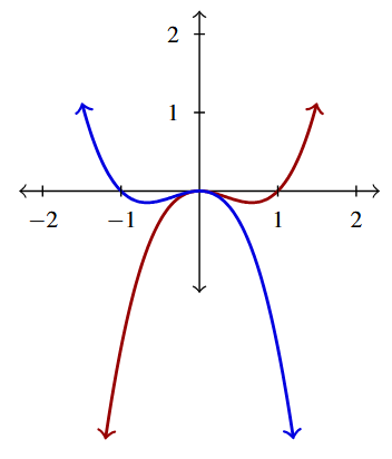
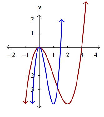
Predict how the graph of [latex]H(s) = 8s^3 - 12s^2[/latex] relates to the graph of [latex]h(s) = s^3-3s^2[/latex] .
Solution:
Predict how the graph of [latex]H(s) = 8s^{3} -12s^{2}[/latex] relates to the graph of [latex]h(s) = s^{3} -3s^{2}[/latex].
When comparing the formulas for [latex]H(s) = 8s^3 - 12s^2[/latex] and [latex]h(s) = s^3-3s^2[/latex], it doesn’t appear as if any shifting or reflecting is going on (why not?)
We also note that the coefficient of [latex]s^3[/latex] in the expression of [latex]H(s)[/latex] is [latex]8[/latex] times that of the coefficient of [latex]s^3[/latex] in [latex]h(s)[/latex], but the coefficient of [latex]s^2[/latex] in [latex]H(s)[/latex] is only [latex]4[/latex] times the coefficient of [latex]s^2[/latex] in [latex]h(s)[/latex], therefore the change is not the result of a vertical scaling (again, why not?)
Hence, if anything, we are looking for a horizontal scaling. In other words, we are looking for a real number [latex]b>0[/latex] so [latex]h(bs) = H(s)[/latex], that is, \[ \begin{array}{rcl} (bs)^3 – 3 (bs)^2 &=& b^3 s^3 – 3b^2 s^2 \\ &=& 8s^3-12s^2 \end{array} \]
Matching up coefficients of [latex]s^3[/latex] gives [latex]b^3=8[/latex] so [latex]b=2[/latex] which checks with the coefficients of [latex]s^2[/latex] : [latex]3b^2 = 3(2)^2 = 12[/latex].
Hence, we predict the graph of [latex]y=H(s)=(2s)^{3}-3(2s)^{2}[/latex] (in blue) to be the same as [latex]y=h(s)=s^{3} - 3s^{2}[/latex] (in red) except horizontally compressed by a factor of 2.
Example 1.6.3.4a
Use Theorems 1.7, 1.8, 1.9, 1.10, and 1.11 to answer the questions below. Check your answers using a graphing utility where appropriate.
Below is the graph of [latex]y = f(x)[/latex].
Use it to sketch the graph of
[latex]F(x) = \dfrac{1-f(x)}{2}[/latex]
Solution:
Sketch the graph of [latex]F(x) = \dfrac{1-f(x)}{2}[/latex].
We first rewrite the expression for [latex]F(x) = \dfrac{1-f(x)}{2} = -\dfrac{1}{2}f(x) + \dfrac{1}{2}[/latex] in order to use the theorems available to us. Note we have two modifications to the formula of [latex]f(x)[/latex] which correspond to three transformations.
Multiplying [latex]f(x)[/latex] by [latex]-\dfrac{1}{2}[/latex] indicates a vertical compression by a factor of 2 along with a reflection about the [latex]x[/latex]-axis. Adding [latex]\dfrac{1}{2}[/latex] indicates a vertical shift up [latex]\dfrac{1}{2}[/latex] units.
As always the question is which to do first. Once again, we look to algebra for the answer. Picking the point [latex](1,0)[/latex] on the graph of [latex]f(x)[/latex], we know [latex]f(1) = 0[/latex]. To see which point this corresponds to on the graph of [latex]y=F(x)[/latex], we find [latex]F(1) = -\dfrac{1}{2}f(1)+\dfrac{1}{2} = -\dfrac{1}{2} (0) +\dfrac{1}{2} = 0 + \dfrac{1}{2} = \dfrac{1}{2}[/latex].
Hence, we first multiplied the [latex]y[/latex]-value 0 by [latex]-\dfrac{1}{2}[/latex]. As above, we can think of [latex]-\dfrac{1}{2} = (-1) \dfrac{1}{2}[/latex] so that multiplying by [latex]-\dfrac{1}{2}[/latex] amounts to a vertical compression by a factor of 2 first, then the reflection about the [latex]x[/latex]-axis second. Lastly, adding the [latex]\dfrac{1}{2}[/latex] is the vertical shift up [latex]\dfrac{1}{2}[/latex] unit.
Beginning with the vertical scaling by a factor of [latex]\dfrac{1}{2}[/latex], we use Theorem 1.10 to graph [latex]y=\dfrac{1}{2} f(x)[/latex] starting from [latex]y=f(x)[/latex] by multiplying each of the [latex]y[/latex]-coordinates of each of the points on the graph of [latex]y=f(x)[/latex] by [latex]\dfrac{1}{2}[/latex].
Next, we reflect the graph of [latex]y = \dfrac{1}{2} f(x)[/latex] across the [latex]x[/latex]-axis to produce the graph of [latex]y=-\dfrac{1}{2} f(x)[/latex] by multiplying each of the [latex]y[/latex]-coordinates of the points on the graph of [latex]y=\dfrac{1}{2} f(x)[/latex] by [latex]-1[/latex]:
Finally, we shift the graph of [latex]y = -\dfrac{1}{2} f(x)[/latex] vertically up [latex]\dfrac{1}{2}[/latex] unit by adding [latex]\dfrac{1}{2}[/latex] to each of the [latex]y[/latex]-coordinates of each of the points to obtain the graph of [latex]y = -\dfrac{1}{2}f(x)+\dfrac{1}{2} = F(x)[/latex].
Note that as with horizontal scalings and reflections about the [latex]y[/latex]-axis, the order of vertical scalings and reflections across the [latex]x[/latex]-axis is interchangeable. Had we decided to think of the factor [latex]-\dfrac{1}{2} = \dfrac{1}{2} \cdot (-1)[/latex], we could have just as well started with the graph of [latex]y=f(x)[/latex] and produced the graph of [latex]y=-f(x)[/latex] first:
Next, we vertically scale the graph of [latex]y=-f(x)[/latex] by multiplying each of the [latex]y[/latex]-coordinates of each of the points on the graph of [latex]y=-f(x)[/latex] by [latex]\dfrac{1}{2}[/latex] to obtain the graph of [latex]y = -\dfrac{1}{2} f(x)[/latex]:
Notice we’ve reached the same graph of [latex]y=-\dfrac{1}{2} f(x)[/latex] that we had before, and, hence we arrive at the same final answer as before:
We check our answer as we have so many times before. We start with the point [latex]\left(1, \dfrac{1}{2}\right)[/latex] and substitute [latex]x=1[/latex] into [latex]y=\dfrac{1-f(x)}{2}[/latex] to get [latex]y=\dfrac{1-f(1)}{2}[/latex]. From the graph of [latex]f[/latex], we know [latex]f(1) = 0[/latex], so we get [latex]y=\dfrac{1-f(1)}{2} = \dfrac{1-0}{2} = \dfrac{1}{2}[/latex]. This proves [latex]\left(1, \dfrac{1}{2}\right)[/latex] is on the graph of [latex]y=\dfrac{1-f(x)}{2}[/latex]. We invite the reader to check the remaining points.
Note that in the preceding example, because none of the transformations included adjusting the [latex]x[/latex]-coordinates of points, the vertical asymptote, [latex]x=0[/latex] remained in place.
Example 1.6.3.4b
Use Theorems 1.7, 1.8, 1.9, 1.10, and 1.11 to answer the questions below. Check your answers using a graphing utility where appropriate.
Below is the graph of [latex]y = f(x)[/latex].
Use it to sketch the graph of
[latex]F(x)= f\left( \dfrac{1-x}{2} \right)[/latex]
Solution:
Sketch the graph of [latex]F(x) = f \left( \dfrac{1-x}{2} \right)[/latex].
As with the previous example, we first rewrite [latex]F(x)= f\left( \dfrac{1-x}{2} \right) = F\left( -\dfrac{1}{2}x + \dfrac{1}{2} \right)[/latex]. Here again, we have two modifications to the formula [latex]f(x)[/latex], the [latex]-\dfrac{1}{2}[/latex] multiple indicating a horizontal scaling and a reflection across the [latex]y[/latex]-axis and a horizontal shift.
Based on our experience from previous examples, we do the horizontal shift first, with the order of the scaling and reflection more or less irrelevant.
To produce the graph of [latex]y = f\left(x+\dfrac{1}{2}\right)[/latex] we subtract [latex]\dfrac{1}{2}[/latex] from each of the [latex]x[/latex]-coordinates of each of the points on the graph of [latex]y=f(x)[/latex]. This moves the graph to the left [latex]\dfrac{1}{2}[/latex] unit, including the vertical asymptote [latex]x=0[/latex] which moves to [latex]x = -\dfrac{1}{2}[/latex].
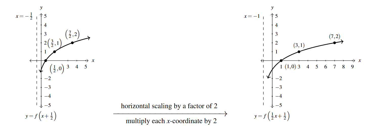
Next, we graph [latex]y = f\left(\dfrac{1}{2}x + \dfrac{1}{2} \right)[/latex] starting with [latex]y = f\left(x+\dfrac{1}{2}\right)[/latex] by horizontally expanding the graph by a factor of 2. That is, we multiply each [latex]x[/latex]-coordinates on the graph of [latex]y = f\left(x+\dfrac{1}{2}\right)[/latex] by 2, including the vertical asymptote, [latex]x =-\dfrac{1}{2}[/latex] which moves to [latex]x = 2 \left(-\dfrac{1}{2} \right) = -1[/latex].
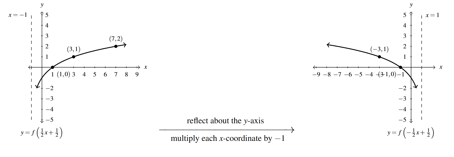
Finally, we reflect the graph of [latex]y = f\left(\dfrac{1}{2}x + \dfrac{1}{2} \right)[/latex] about the [latex]y[/latex]-axis to graph [latex]y = f\left(-\dfrac{1}{2}x + \dfrac{1}{2} \right)[/latex]. We accomplish this by multiplying each of the [latex]x[/latex]-coordinates of each of the points on the graph of [latex]y = f\left(\dfrac{1}{2}x + \dfrac{1}{2} \right)[/latex] by [latex]-1[/latex]. This includes the vertical asymptote which is moved to [latex]x = (-1)(-1) = 1[/latex].
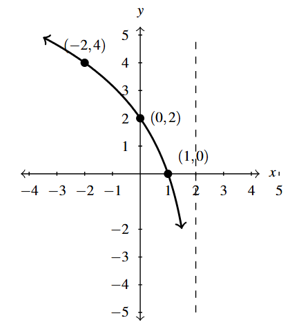
To check our answer, we begin with the point [latex](-1,0)[/latex] and substitute [latex]x=-1[/latex] into [latex]y = f\left( \dfrac{1-x}{2} \right)[/latex]. We get [latex]y = f\left( \dfrac{1-(-1)}{2} \right) = f\left( \dfrac{2}{2} \right) = f(1)[/latex]. From the graph of [latex]f[/latex], we know [latex]f(1) = 0[/latex], hence we have [latex]y = f(1) = 0[/latex], proving [latex](-1,0)[/latex] is on the graph of [latex]y = f\left( \dfrac{1-x}{2}\right)[/latex]. The reader is encouraged to check the remaining points.
As mentioned previously, instead of doing the horizontal scaling first, then the reflection, we could have done the reflection first, then the scaling. We leave this to the reader to check.
Example 1.6.3.5
Use Theorems 1.7, 1.8, 1.9, 1.10, and 1.11 to answer the questions below. Check your answers using a graphing utility where appropriate.
Below is the graph of [latex]y = g(x)[/latex]. Write [latex]g(x)[/latex] in terms of [latex]f(x)[/latex] from part 4 and vice-versa.
NOTE: The [latex]y[/latex]-axis, [latex]x=0[/latex], is a vertical asymptote to the graph of [latex]y = f(x)[/latex] and the line [latex]x=2[/latex] is a vertical asymptote to the graph of [latex]y = g(x)[/latex].
Solution:
Write [latex]g(x)[/latex] in terms of [latex]f(x)[/latex] and visa-versa.
To write [latex]g(x)[/latex] in terms of [latex]f(x)[/latex], we assume we can find real numbers [latex]a[/latex], [latex]b[/latex], [latex]h[/latex], and [latex]k[/latex] and choose signs [latex]\pm[/latex] so that [latex]g(x) = \pm a f(\pm b x - h)+k[/latex].
The most notable change we see is the vertical asymptote [latex]x=0[/latex] has moved to [latex]x=2[/latex]. Moreover, instead of the graph increasing off to the right, it is decreasing coming in from the left. This suggests a horizontal shift of 2 units as well as a reflection across the [latex]y[/latex]-axis.
We always shift first and then reflect, so we have a shift left of 2 units followed by a reflection about the [latex]y[/latex]-axis. In other words, [latex]g(x) = \pm a f(-x+2) + k[/latex].
Comparing [latex]y[/latex]-values, the [latex]y[/latex]-values on the graph of [latex]g[/latex] appear to be exactly twice the corresponding values on the graph of [latex]f[/latex], indicating a vertical stretch by a factor of 2. Hence, we get [latex]g(x) = 2 f(-x+2)[/latex]. We leave it to the reader to check the graph of [latex]y=2f(-x+2)[/latex] matches the graph of [latex]y=g(x)[/latex].
To write [latex]f(x)[/latex] in terms of [latex]g(x)[/latex], we reverse the steps done in obtaining the graph of [latex]g(x)[/latex] from [latex]f(x)[/latex] in the reverse order.
To get from the graph of [latex]f[/latex] to the graph of [latex]g[/latex], we: first, shifted left 2 units; second reflected across the [latex]y[/latex]-axis; third, vertically stretched by a factor of 2, thus our first step in taking [latex]g[/latex] back to [latex]f[/latex] is to implement a vertical compression by a factor of 2. Hence, starting with the graph of [latex]y=g(x)[/latex], our first step results in the formula [latex]y = \dfrac{1}{2} g(x)[/latex].
Next, we need to undo the reflection about the [latex]y[/latex]-axis. If the point [latex](a,b)[/latex] is reflected about the [latex]y[/latex]-axis, we obtain the point [latex](-a,b)[/latex]. To return to the point [latex](a,b)[/latex], we reflect [latex](-a,b)[/latex] across the [latex]y[/latex]-axis again: [latex](-(-a),b) = (a,b)[/latex]. Hence, we take the graph of [latex]y = \dfrac{1}{2} g(x)[/latex] and reflect it across the [latex]y[/latex]-axis to obtain [latex]y = \dfrac{1}{2} g(-x)[/latex].
Our last step is to undo a horizontal shift to the left 2 units. The reverse of this process is shifting the graph to the right two units, so we get [latex]y = \dfrac{1}{2} g(-(x-2)) = \dfrac{1}{2} g(-x+2)[/latex].[12]
We leave it to the reader to start with the graph of [latex]y=g(x)[/latex] and check the graph of [latex]y = \dfrac{1}{2} g(-x+2)[/latex] matches the graph of [latex]y = f(x)[/latex].
1.6.4 Transformations in Sequence
Now that we have studied three basic classes of transformations: shifts, reflections, and scalings, we present a result below which provides one algorithm to follow to transform the graph of [latex]y=f(x)[/latex] into the graph of [latex]y=a \, f(bx-h)+k[/latex] without the need of using Theorems 1.7, 1.8, 1.9, 1.10, and 1.11 individually.
Theorem 1.12 is the ultimate generalization of Theorems 1.4, 2.1, 2.2, 3.1, 4.1 and 4.4. We note the underlying assumption here is that regardless of the order or number of shifts, reflections and scalings applied to the graph of a function [latex]f[/latex], we can always represent the final result in the form [latex]g(x) = a \, f(bx-h)+k[/latex]. Each of these transformations can ultimately be traced back to composing [latex]f[/latex] with linear functions,[13] this fact is verified by showing compositions of linear functions results in a linear function.
Suppose [latex]f[/latex] is a function. If [latex]a, b \neq 0[/latex], then to graph [latex]g(x) = a \, f(bx-h)+k[/latex] start with the graph of [latex]y=f(x)[/latex] and follow the steps below.
- Add [latex]h[/latex] to each of the [latex]x[/latex]-coordinates of the points on the graph of [latex]f[/latex].
NOTE: This results in a horizontal shift to the left if [latex]h[/latex] < [latex]0[/latex] or right if [latex]h > 0[/latex]. - Divide the [latex]x[/latex]-coordinates of the points on the graph obtained in Step 1 by [latex]b[/latex].
NOTE: This results in a horizontal scaling, but includes a reflection about the [latex]y[/latex]-axis if [latex]b[/latex] < [latex]0[/latex]. - Multiply the [latex]y[/latex]-coordinates of the points on the graph obtained in Step 2 by [latex]a[/latex].
NOTE: This results in a vertical scaling, but includes a reflection about the [latex]x[/latex]-axis if [latex]a[/latex] < [latex]0[/latex]. - Add [latex]k[/latex] to each of the [latex]y[/latex]-coordinates of the points on the graph obtained in Step 3.
NOTE: This results in a vertical shift up if [latex]k > 0[/latex] or down if [latex]k[/latex] < [latex]0[/latex].
Theorem 1.12 can be established by generalizing the techniques developed in this section. Suppose [latex](c,f(c))[/latex] is on the graph of [latex]f[/latex]. To match up the inputs of [latex]f(bx-h)[/latex] and [latex]f(c)[/latex], we solve [latex]bx-h = c[/latex] and solve.
We first add the [latex]h[/latex] (causing the horizontal shift) and then divide by [latex]b[/latex]. If [latex]b[/latex] is a positive number, this induces only a horizontal scaling by a factor of [latex]\dfrac{1}{b}[/latex]. If [latex]b[/latex] < [latex]0[/latex], then we have a factor of [latex]-1[/latex] in play, and dividing by it induces a reflection about the [latex]y[/latex]-axis. So we have [latex]x = \dfrac{c+h}{b}[/latex] as the input to [latex]g[/latex] which corresponds to the input [latex]x=c[/latex] to [latex]f[/latex].
We now evaluate [latex]g\left( \dfrac{c+h}{b}\right) = a \, f\left(b \cdot \dfrac{c+h}{b} -h \right) + k = a \, f(c+h-h) = a \, f(c)+k[/latex]. We notice that the output from [latex]f[/latex] is first multiplied by [latex]a[/latex]. As with the constant [latex]b[/latex], if [latex]a > 0[/latex], this induces only a vertical scaling. If [latex]a[/latex] < [latex]0[/latex], then the [latex]-1[/latex] induces a reflection across the [latex]x[/latex]-axis. Finally, we add [latex]k[/latex] to the result, which is our vertical shift.
A less precise, but more intuitive way to paraphrase Theorem 1.12 is to think of the quantity [latex]bx-h[/latex] is the inside of the function [latex]f[/latex]. What’s happening inside [latex]f[/latex] affects the inputs or [latex]x[/latex]-coordinates of the points on the graph of [latex]f[/latex]. To find the [latex]x[/latex]-coordinates of the corresponding points on [latex]g[/latex], we undo what has been done to [latex]x[/latex] in the same way we would solve an equation.
What’s happening to the output can be thought of as things happening outside the function, [latex]f[/latex]. Things happening outside affect the outputs or [latex]y[/latex]-coordinates of the points on the graph of [latex]f[/latex]. Here, we follow the usual order of operations to simplify the new [latex]y[/latex]-value: we first multiply by [latex]a[/latex], then add [latex]k[/latex] to find the corresponding [latex]y[/latex]-coordinates on the graph of [latex]g[/latex].
It needs to be stressed that our approach to handling multiple transformations, as summarized in Theorem 1.12 is only one approach. There are various algorithm that can be used. As always, the more you understand, the less you’ll ultimately need to memorize, so whatever algorithm you choose to follow, it is worth thinking through each step both algebraically and geometrically.
We make good use of Theorem 1.12 in the following example.
Example 1.6.4
Example 1.6.4
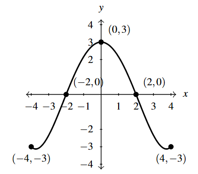
Below is the complete graph of [latex]y = f(x)[/latex]. Use Theorem 1.12 to graph [latex]g(x) = \dfrac{4-3 f(1-2x)}{2}[/latex].
Solution:
We use Theorem 1.12 to track the five key points [latex](-4,-3)[/latex], [latex](-2,0)[/latex], [latex](0,3)[/latex], [latex](2,0)[/latex] and [latex](4,-3)[/latex] indicated on the graph of [latex]f[/latex] to their new locations.
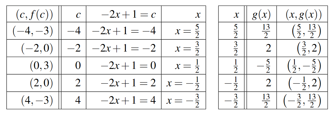
We first rewrite [latex]g(x)[/latex] in the form presented in Theorem 1.12, [latex]g(x) = -\dfrac{3}{2}f(-2x+1) +2[/latex]. We set [latex]-2x+1[/latex] equal each of the [latex]x[/latex]-coordinates of the key points and solve.
For example, solving [latex]-2x+1 = -4[/latex], we first subtract 1 to get [latex]-2x = -5[/latex] then divide by [latex]-2[/latex] to get [latex]x = \dfrac{5}{2}[/latex]. Subtracting the 1 is a horizontal shift to the left 1 unit. Dividing by [latex]-2[/latex] can be thought of as a two step process: dividing by 2 which compresses the graph horizontally by a factor of 2 followed by dividing (multiplying) by [latex]-1[/latex] which causes a reflection across the [latex]y[/latex]-axis. We summarize the results in a table below on the left.
Next, we take each of the [latex]x[/latex] values and substitute them into [latex]g(x) = -\dfrac{3}{2}f(-2x+1) +2[/latex] to get the corresponding [latex]y[/latex]-values. Substituting [latex]x=\dfrac{5}{2}[/latex], and using the fact that [latex]f(-4)=-3[/latex], we get \[\begin{array}{rcl} g\left(\dfrac{5}{2}\right) &=& -\dfrac{3}{2}f\left(-2\left(\dfrac{5}{2}\right) +1\right) +2 \\ &=& -\dfrac{3}{2} f(-4) + 2 \\ &=& -\dfrac{3}{2}(-3) + 2 \\ &=& \dfrac{9}{2} + 2 \\ &=& \dfrac{13}{2} \end{array} \] We see that the output from [latex]f[/latex] is first multiplied by [latex]-\dfrac{3}{2}[/latex]. Thinking of this as a two step process, multiplying by [latex]\dfrac{3}{2}[/latex] then by [latex]-1[/latex], we have a vertical stretching by a factor of [latex]\dfrac{3}{2}[/latex] followed by a reflection across the [latex]x[/latex]-axis. Adding 2 results in a vertical shift up 2 units. Continuing in this manner, we get the table below on the right.
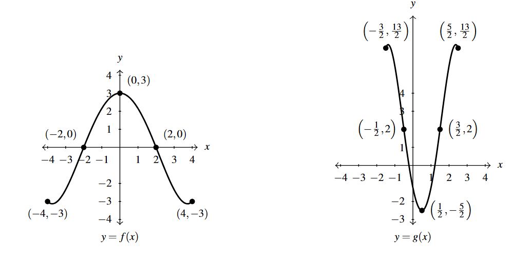
To graph [latex]g[/latex], we plot each of the points in the table above and connect them in the same order and fashion as the points to which they correspond. Plotting [latex]f[/latex] and [latex]g[/latex] side-by-side gives
The reader is strongly encouraged to graph the series of functions which shows the gradual transformation of the graph of [latex]f[/latex] into the graph of [latex]g[/latex] in Example 1.6.4. We have outlined the sequence of transformations in the above exposition; all that remains is to plot the five intermediate stages.
Our next example turns the tables and asks for the formula of a function given a desired sequence of transformations.
Example 1.6.5
Example 1.6.5
Let [latex]f(x) = x^2 - |x|[/latex]. Construct and simplify the formula of the function [latex]g(x)[/latex] whose graph is the result of the graph of [latex]y=f(x)[/latex] undergoing the following sequence of transformations. Check your answer to each step using a graphing utility.
- Vertical shift up 2 units.
- Reflection across the [latex]x[/latex]-axis.
- Horizontal shift right 1 unit.
- Horizontal compression by a factor of 2.
- Vertical shift up 3 units.
- Reflection across the [latex]y[/latex]-axis.
Solution:
To help keep us organized we will label each intermediary function. The function [latex]g_{1}[/latex] will be the result of applying the first transformation to [latex]f[/latex]. The function [latex]g_{2}[/latex] will be the result of applying the first two transformations to [latex]f[/latex] – which is also the result of applying the second transformation to [latex]g_{1}[/latex], and so on.[14]
- Per Theorem 1.7, [latex]g_{1}(x) = f(x) + 2 = x^2-|x|+2[/latex] (in red).
First Step of Example 1.6.5 - Per Theorem 1.9, [latex]g_{2}(x) = -g_{1}(x) = -[x^2-|x|+2] = -x^2+|x|-2[/latex] (in blue).
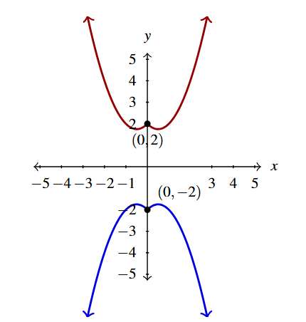
Second Step of Example 1.6.5 - Per Theorem 1.8, [latex]g_{3}(x) = g_{2}(x-1) = -(x-1)^2+|x-1|-2[/latex] (in red).
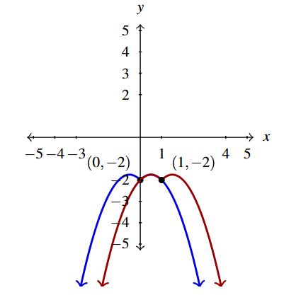
Third Step of Example 1.6.5 - Per Theorem 1.11, [latex]g_{4}(x) = g_{3}(2x) = -(2x-1)^2+|2x-1| - 2[/latex] (in blue).
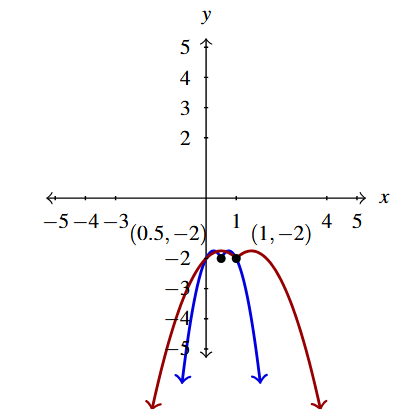
Fourth Step in Example 1.6.5 - Per Theorem 1.7, [latex]g_{5}(x) = g_{4}(x)+3 = -(2x-1)^2+|2x-1| - 2 + 3 = -(2x-1)^2+|2x-1| +1[/latex] (in red).
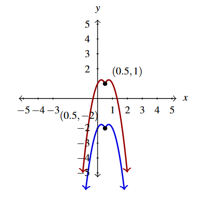
Fifth Step of Example 1.6.5 - Per Theorem 1.9, [latex]g_{6}(x) = g_{5}(-x)[/latex] (in blue): \[ \begin{array}{rcl}
g_{6}(x) & = & g_{5}(-x) \\
& = & -(2(-x)-1)^2+|2(-x)-1|+1 \\
& = & -(-2x-1)^2+|-2x-1|+1 \\
& = & -[(-1)(2x+1)]^2+|[(-1)(2x+1)|+1 \\
& = & -(-1)^2(2x+1)^2+|-1||2x+1| + 1 \\
& = & -(2x+1)^2+|2x+1|+1 \\
\end{array} \]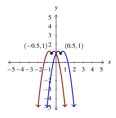
Last Step of Example 1.6.5
Hence, [latex]g(x) = g_{6}(x) = -(2x+1)^2+|2x+1| + 1[/latex].
It is instructive to show that the expression [latex]g(x)[/latex] in Example 1.6.4 can be written as [latex]g(x) = a \, f(bx-h)+k[/latex].
One way is to compare the graphs of [latex]f[/latex] and [latex]g[/latex] and work backwards. A more methodical way is to repeat the work of Example 1.6.4, but never substitute the formula for [latex]f(x)[/latex] as follows:
- Per Theorem 1.7, [latex]g_{1}(x) = f(x) + 2[/latex].
- Per Theorem 1.9, [latex]g_{2}(x) = -g_{1}(x) = -[f(x) + 2] = -f(x)-2[/latex].
- Per Theorem 1.8, [latex]g_{3}(x) = g_{2}(x-1) = -f(x-1)-2[/latex].
- Per Theorem 1.11, [latex]g_{4}(x) = g_{3}(2x) =-f(2x-1)-2[/latex].
- Per Theorem 1.7, [latex]g_{5}(x) = g_{4}(x)+3 = -f(2x-1)-2 + 3 = -f(2x-1)+1[/latex].
- Per Theorem 1.9, [latex]g_{6}(x) = g_{5}(-x) = -f(2(-x)-1)+1 = -f(-2x-1)+1[/latex].
Hence [latex]g(x) = -f(-2x-1)+1[/latex]. Note we can show [latex]f[/latex] is even,[15] so [latex]f(-2x-1) = f(-(2x+1)) = f(2x+1)[/latex] and obtain [latex]g(x) = -f(2x+1)+1[/latex].
At the beginning of this section, we discussed how all of the transformations we’d be discussing are the result of composing given functions with linear functions. Not all transformations, not even all rigid transformations, fall into these categories.
For example, consider the graphs of [latex]y=f(x)[/latex] and [latex]y=g(x)[/latex] below.
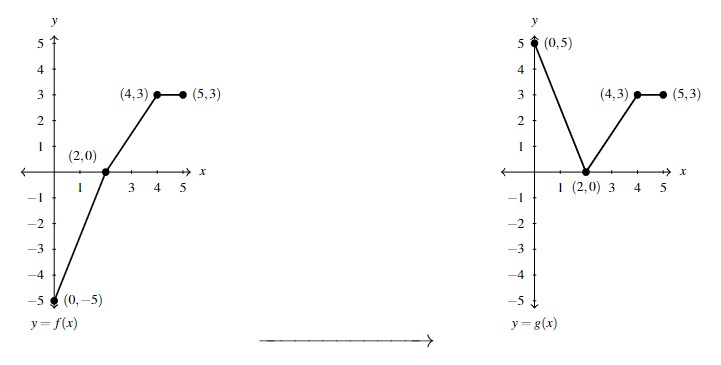
In Exercise 76, we explore a non-linear transformation and revisit the pair of functions [latex]f[/latex] and [latex]g[/latex] then.
1.6.5 Section Exercises
Suppose [latex](2,-3)[/latex] is on the graph of [latex]y = f(x)[/latex]. In Exercises 1 – 18, use Theorem 1.12 to find a point on the graph of the given transformed function.
- [latex]y = f(x)+3[/latex]
- [latex]y = f(x+3)[/latex]
- [latex]y = f(x)-1[/latex]
- [latex]y = f(x-1)[/latex]
- [latex]y = 3f(x)[/latex]
- [latex]y = f(3x)[/latex]
- [latex]y = -f(x)[/latex]
- [latex]y = f(-x)[/latex]
- [latex]y = f(x-3)+1[/latex]
- [latex]y = 2f(x+1)[/latex]
- [latex]y = 10 - f(x)[/latex]
- [latex]y = 3f(2x) - 1[/latex]
- [latex]y = \dfrac{1}{2} f(4-x)[/latex]
- [latex]y = 5f(2x+1) + 3[/latex]
- [latex]y = 2f(1-x) -1[/latex]
- [latex]y =f\left(\dfrac{7-2x}{4}\right)[/latex]
- [latex]y = \dfrac{f(3x) - 1}{2}[/latex]
- [latex]y = \dfrac{4-f(3x-1)}{7}[/latex]
The complete graph of [latex]y = f(x)[/latex] is given below. In Exercises 19 – 27, use it and Theorem 1.12 to graph the given transformed function.
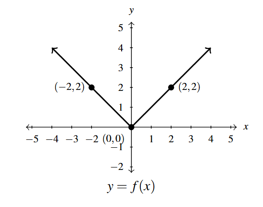
- [latex]y = f(x) + 1[/latex]
- [latex]y = f(x) - 2[/latex]
- [latex]y = f(x+1)[/latex]
- [latex]y = f(x - 2)[/latex]
- [latex]y = 2f(x)[/latex]
- [latex]y = f(2x)[/latex]
- [latex]y = 2 - f(x)[/latex]
- [latex]y = f(2-x)[/latex]
- [latex]y = 2-f(2-x)[/latex]
- Some of the answers to Exercises 19 – 27 above should be the same. Which ones match up? What properties of the graph of [latex]y=f(x)[/latex] contribute to the duplication?
- The function [latex]f[/latex] used in Exercises 19- 27 should look familiar. What is [latex]f(x)[/latex]? How does this this explain some of the duplication in the answers to Exercises 19 – 27 mentioned in Exercise 28?
The complete graph of [latex]y =g(t)[/latex] is given below. In Exercises 30 – 38, use it and Theorem 1.12 to graph the given transformed function.
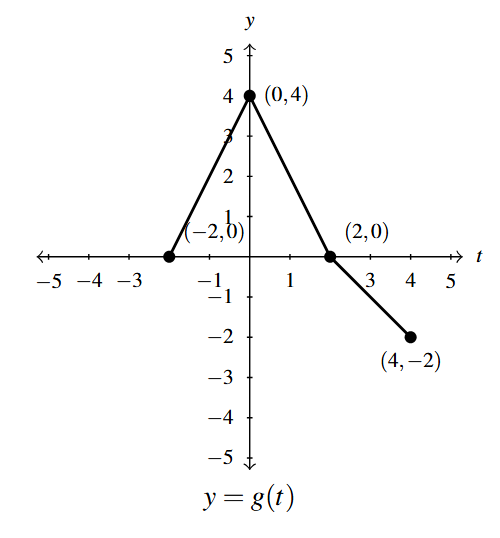
- [latex]y = g(t) - 1[/latex]
- [latex]y = g(t + 1)[/latex]
- [latex]y = \dfrac{1}{2} g(t)[/latex]
- [latex]y = g(2t)[/latex]
- [latex]y = - g(t)[/latex]
- [latex]y = g(-t)[/latex]
- [latex]y = g(t+1) - 1[/latex]
- [latex]y = 1 - g(t)[/latex]
- [latex]y = \dfrac{1}{2}g(t+1)-1[/latex]
The complete graph of [latex]y = f(x)[/latex] is given below. In Exercises 39 – 50, use it and Theorem 1.12 to graph the given transformed function.
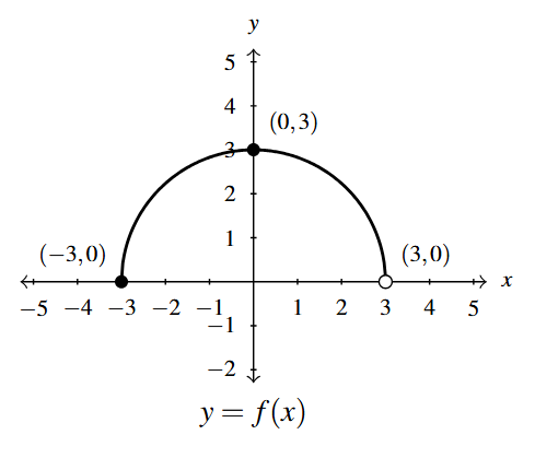
- [latex]g(x) = f(x) + 3[/latex]
- [latex]h(x) = f(x) - \dfrac{1}{2}[/latex]
- [latex]j(x) = f\left(x - \dfrac{2}{3}\right)[/latex]
- [latex]a(x) = f(x + 4)[/latex]
- [latex]b(x) = f(x + 1) - 1[/latex]
- [latex]c(x) = \dfrac{3}{5}f(x)[/latex]
- [latex]d(x) = -2f(x)[/latex]
- [latex]k(x) = f\left(\dfrac{2}{3}x\right)[/latex]
- [latex]m(x) = -\dfrac{1}{4}f(3x)[/latex]
- [latex]n(x) = 4f(x - 3) - 6[/latex]
- [latex]p(x) = 4 + f(1 - 2x)[/latex]
- [latex]q(x) = -\dfrac{1}{2}f\left(\dfrac{x + 4}{2}\right) - 3[/latex]
The complete graph of [latex]y = S(t)[/latex] is given below.
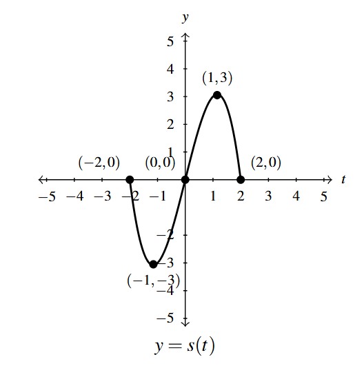
The purpose of Exercises 51 – 54 is to build up to the graph of [latex]y = \dfrac{1}{2}S(-t+1) + 1[/latex] one step at a time.
- [latex]y = S_{1}(t) = S(t + 1)[/latex]
- [latex]y = S_{2}(t) = S_{1}(-t) = S(-t + 1)[/latex]
- [latex]y = S_{3}(t) = \dfrac{1}{2} S_{2}(t) = \dfrac{1}{2}S(-t+1)[/latex]
- [latex]y = S_{4}(t) = S_{3}(t) + 1 = \dfrac{1}{2}S(-t+1) + 1[/latex]
For Exercises 55 – 64 let [latex]f(x) = \sqrt{x}[/latex]. Find a formula for a function [latex]g[/latex] whose graph is obtained from [latex]f[/latex] from the given sequence of transformations.
- (1) shift right 2 units; (2) shift down 3 units
- (1) shift down 3 units; (2) shift right 2 units
- (1) reflect across the [latex]x[/latex]-axis; (2) shift up 1 unit
- (1) shift up 1 unit; (2) reflect across the [latex]x[/latex]-axis
- (1) shift left 1 unit; (2) reflect across the [latex]y[/latex]-axis; (3) shift up 2 units
- (1) reflect across the [latex]y[/latex]-axis; (2) shift left 1 unit; (3) shift up 2 units
- (1) shift left 3 units; (2) vertical stretch by a factor of 2; (3) shift down 4 units
- (1) shift left 3 units; (2) shift down 4 units; (3) vertical stretch by a factor of 2
- (1) shift right 3 units; (2) horizontal shrink by a factor of 2; (3) shift up 1 unit
- (1) horizontal shrink by a factor of 2; (2) shift right 3 units; (3) shift up 1 unit
For Exercises 65 – 70, use the given of [latex]y = f(x)[/latex] to write each function in terms of [latex]f(x)[/latex].
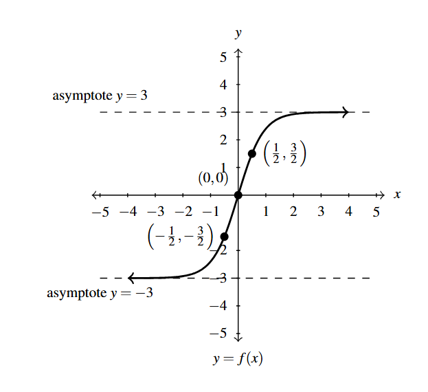
- [latex]y = g(x)[/latex] with asymptotes of [latex]y = 4[/latex] and [latex]y = -2[/latex]
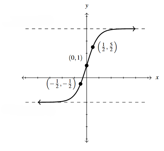
Graph of Exercise 65 - [latex]y = h(x)[/latex] with asymptotes of [latex]y = 3[/latex] and [latex]y = -3[/latex]
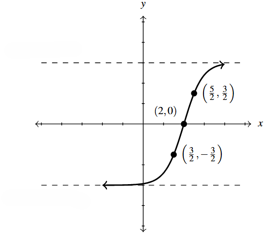
Graph for Exercise 66 - [latex]y = p(x)[/latex] with asymptotes of [latex]y = 2[/latex] and [latex]y = -4[/latex]
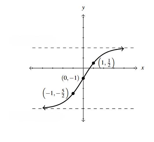
Graph for Exercise 67 - [latex]y = q(x)[/latex] with asymptotes of [latex]y = 6[/latex] and [latex]y = -6[/latex]
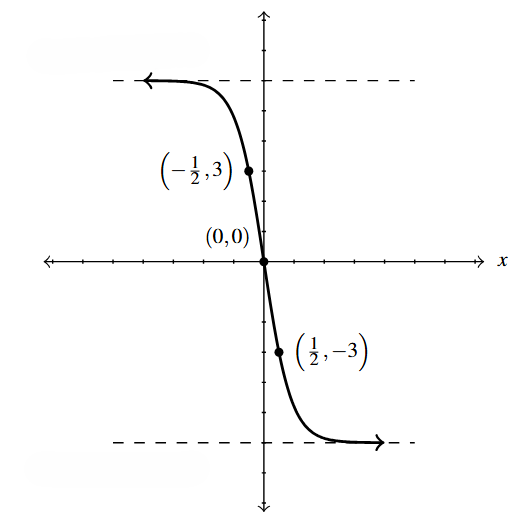
Graph for Exercise 68 - [latex]y = r(x)[/latex] with asymptotes of [latex]y = 3[/latex] and [latex]y = -9[/latex]
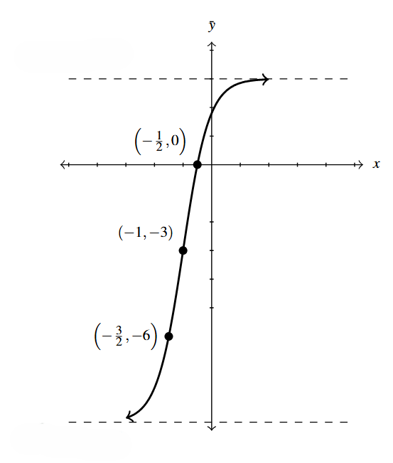
Graph for Exercise 69 - [latex]y = s(x)[/latex] with asymptotes of [latex]y = 3[/latex] and [latex]y = -9[/latex]
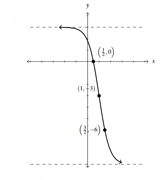
Graph for Exercise 70 - The graph of [latex]y = f(x) = \sqrt[3]{x}[/latex] is given below on the left and the graph of [latex]y = g(x)[/latex] is given on the right. Find a formula for [latex]g[/latex] based on transformations of the graph of [latex]f[/latex]. Check your answer by confirming that the points shown on the graph of [latex]g[/latex] satisfy the equation [latex]y = g(x)[/latex].
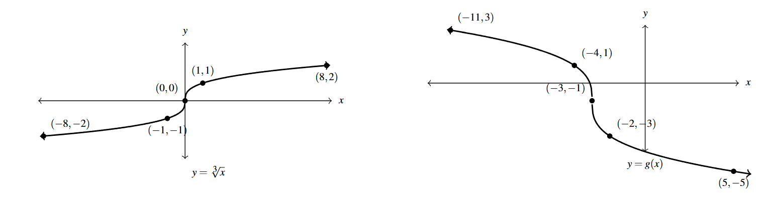
Graphs for Exercise 71 - Show that the composition of two linear functions is a linear function. Hence any (finite) sequence of transformations discussed in this section can be combined into the form given in Theorem 1.12.
(HINT: Let [latex]f(x) = ax +b[/latex] and [latex]g(x) = cx + d[/latex]. Find [latex](f \circ g)(x)[/latex].) - For many common functions, the properties of Algebra make a horizontal scaling the same as a vertical scaling by (possibly) a different factor. For example, [latex]\sqrt{9x} = 3\sqrt{x}[/latex], so a horizontal compression of [latex]y = \sqrt{x}[/latex] by a factor of [latex]9[/latex] results in the same graph as a vertical stretch of [latex]y = \sqrt{x}[/latex] by a factor of 3.
With the help of your classmates, find the equivalent vertical scaling produced by the horizontal scalings [latex]y = (2x)^{3}, \, y = |5x|, \, y = \sqrt[3]{27x} \,[/latex] and [latex]\, y = \left(\dfrac{1}{2} x\right)^{2}[/latex].
What about [latex]y = (-2x)^{3}, \, y = |-5x|, \, y = \sqrt[3]{-27x}\,[/latex] and [latex]\, y = \left(-\dfrac{1}{2} x\right)^{2}[/latex]? - Discuss the following questions with your classmates.If [latex]f[/latex] is even, what happens when you reflect the graph of [latex]y = f(x)[/latex] across the [latex]y[/latex]-axis?
- If [latex]f[/latex] is odd, what happens when you reflect the graph of [latex]y = f(x)[/latex] across the [latex]y[/latex]-axis?
- If [latex]f[/latex] is even, what happens when you reflect the graph of [latex]y = f(x)[/latex] across the [latex]x[/latex]-axis?
- If [latex]f[/latex] is odd, what happens when you reflect the graph of [latex]y = f(x)[/latex] across the [latex]x[/latex]-axis?
- How would you describe symmetry about the origin in terms of reflections?
- We mentioned earlier in the section that, in general, the order in which transformations are applied matters, yet in our first example with two transformations the order did not matter. (You could perform the shift to the left followed by the shift down or you could shift down and then left to achieve the same result.) With the help of your classmates, determine the situations in which order does matter and those in which it does not.
- This Exercise is a follow-up to Exercise 11 in Section 1.4.
- For each of the following functions, use a graphing utility to compare the graph of [latex]y = f(x)[/latex] with the graphs of [latex]y = |f(x)|[/latex] and [latex]y = f(|x|)[/latex].
- [latex]f(x) = 3-x[/latex]
- [latex]f(x) = x^2-x-6[/latex]
- [latex]f(x) = \sqrt{x+3} - 1[/latex]
- In general, how does the graph of [latex]y = |f(x)|[/latex] compare with that of [latex]y = f(x)[/latex]? What about the graph of [latex]y = f(|x|)[/latex] and [latex]y = f(x)[/latex]?
- Referring to the functions [latex]f[/latex] and [latex]g[/latex] graphed right before the Exercises, write [latex]g[/latex] in terms of [latex]f[/latex].
- For each of the following functions, use a graphing utility to compare the graph of [latex]y = f(x)[/latex] with the graphs of [latex]y = |f(x)|[/latex] and [latex]y = f(|x|)[/latex].
Section 1.6 Exercise Answers can be found in the Appendix.
- We'll have more to say about this sort of thing in Section 5.1. ↵
- To see this better, let us temporarily write [latex]F(x) = g(x)-4[/latex]. Theorem 1.9 tells us to reflect the graph of [latex]F[/latex] about the [latex]x[/latex]-axis, graph [latex]y=-F(x) = - [g(x)-4] = -g(x)+4[/latex]. ↵
- Another word that can be used here instead of rigid transformation is isometry - meaning same distance. ↵
- Also called a vertical stretch, vertical expansion or vertical dilation by a factor of 2. ↵
- Also called vertical shrink, vertical compression or vertical contraction by a factor of 2. ↵
- expansion, dilation ↵
- compression, contraction ↵
- Also called horizontal shrink, horizontal compression or horizontal contraction by a factor of 2. ↵
- Also called horizontal stretch, horizontal expansion or horizontal dilation by a factor of 2. ↵
- expansion, dilation ↵
- compression, contraction ↵
- To see this better, let [latex]F(x) = \dfrac{1}{2} g(-x)[/latex]. Per Theorem 1.8, the graph of [latex]F(x-2) = \dfrac{1}{2} g(-(x-2)) = \dfrac{1}{2} g(-x+2)[/latex] is the same as the graph of [latex]F[/latex] but shifted 2 units to the right. ↵
- See the remarks at the beginning of the section. ↵
- So, we can think of [latex]g_{0} = f[/latex] and [latex]g_{6} = g[/latex]. ↵
- Recall this means [latex]f(-x) = f(x)[/latex]. ↵
Rigid transformations are changes to the graph which do not change the shape of the graph, only the position in the plane.
