
4.1 Properties of Root Functions and Their Graphs
As with polynomial functions and rational functions, we begin our study of functions involving radicals with a special family of functions: the (principal) root functions.
4.1.1 Root Functions
Let [latex]n \in \mathbb{N}[/latex] with [latex]n \geq 2[/latex]. The [latex]n[/latex]th (principal) root function is the function [latex]f(x) = \sqrt[n]{x}[/latex].
NOTE: If [latex]n[/latex] is even, the domain of [latex]f[/latex] is [latex][0, \infty)[/latex]; if [latex]n[/latex] is odd, the domain of [latex]f[/latex] is [latex](-\infty, \infty)[/latex].
The domain restriction for even indexed roots means that, once again, we are restricting our attention to real numbers.[1] We graph a few members of the root function family below, and quickly notice that, as with the monomial, and, more generally, the Laurent monomial functions, the behavior of the root functions depends primarily on whether the root is even or odd.
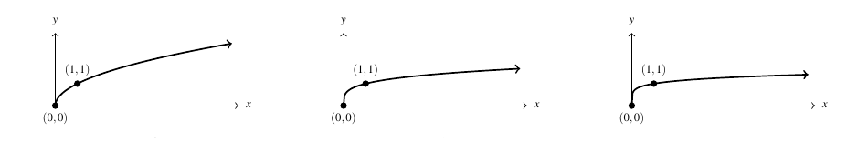
In addition to having the common domain of [latex][0, \infty)[/latex], the graphs of [latex]f(x) = \sqrt[n]{x}[/latex] for even indices, [latex]n[/latex], all share the points [latex](0,0)[/latex] and [latex](1,1)[/latex]. As [latex]n[/latex] increases, the functions become steeper near the [latex]y[/latex]-axis and flatter as [latex]x \rightarrow \infty[/latex]. To show [latex]f(x) \rightarrow \infty[/latex] as [latex]x \rightarrow \infty[/latex], we show, more generally, the range of [latex]f[/latex] is [latex][0, \infty)[/latex]. Indeed, if [latex]c \geq 0[/latex] is a real number, then [latex]f(c^n) = \sqrt[n]{c^n} = c[/latex] so [latex]c[/latex] is in the range of [latex]f[/latex]. Note that [latex]f[/latex] is increasing: that is, if [latex]a[/latex] < [latex]b[/latex], then [latex]f(a) = \sqrt[n]{a}[/latex] < [latex]\sqrt[n]{b} = f(b)[/latex]. This property is useful in solving certain types of polynomial inequalities.[2]
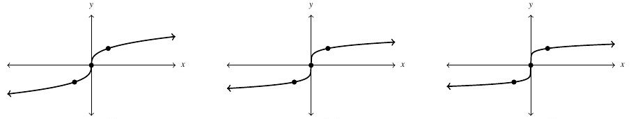
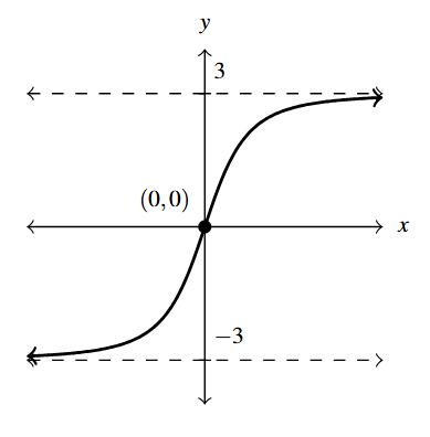
The functions [latex]f(x) = \sqrt[n]{x}[/latex] for odd natural numbers, [latex]n \geq 3[/latex], also follow a predictable trend – steepening near [latex]x = 0[/latex] and flattening as [latex]x \rightarrow \pm \infty[/latex]. The range for these functions is [latex](-\infty, \infty)[/latex] because if [latex]c[/latex] is any real number, [latex]f(c^n) = \sqrt[n]{c^n} = c[/latex], so [latex]c[/latex] is in the range of [latex]f[/latex]. Like the even indexed roots, the odd indexed roots are also increasing. Moreover, these graphs appear to be symmetric about the origin. Sure enough, when [latex]n[/latex] is odd, [latex]f(-x) = \sqrt[n]{-x} = -\sqrt[n]{x} = -f(x)[/latex] so [latex]f[/latex] is an odd function.
At this point, you’re probably expecting a theorem like Theorem 1.12 – that is, a theorem which tells us how to obtain the graph of [latex]F(x) = a \sqrt[n]{x-h}+k[/latex] from the graph of [latex]f(x) = \sqrt[n]{x}[/latex] – and you would not be wrong. Here, however, we need to add an extra parameter [latex]b[/latex] to the recipe and discuss functions of the form [latex]F(x) = a \sqrt[n]{bx-h}+k[/latex]. The reason is that, with all of the previous function families, we were always able to factor out the coefficient of [latex]x[/latex]. We list some examples of this below, and invite the reader to revisit other examples in the text:
- [latex]F(x) = |6-2x| = |-2x+6| = |-2(x-3)| = |-2||x-3| = 2 |x-3|[/latex]
- [latex]\begin{array}{rcl} F(x) = (2x-1)^2 + 1 &=& \left[2 \left(x - \dfrac{1}{2}\right)\right]^2+1 \\ &=& (2)^2 \left(x - \dfrac{1}{2}\right)^2 + 1 \\ &=& 4\left(x - \dfrac{1}{2}\right)^2 + 1 \end{array}[/latex]
- [latex]\begin{array}{rcl} F(x) = \dfrac{2}{(1-x)^3}- 5 &=& \dfrac{2}{[(-1)(x-1)]^3} - 5 \\ &=& \dfrac{2}{(-1)^3(x-1)^3} - 5\\ &=& \dfrac{2}{- (x-1)^3} - 5 \\ &=& \dfrac{-2}{(x-1)^3} - 5 \end{array}[/latex]
For a function like [latex]F(x) = \sqrt{4x-12} + 1 = \sqrt{4(x-6)} + 1 = \sqrt{4}\sqrt{x-3} + 1 = 2 \sqrt{x-3} + 1[/latex], this approach works fine. However, if the coefficient of [latex]x[/latex] is negative, for example, [latex]F(x) = \sqrt{1-x} = \sqrt{(-1)(x-1)}[/latex] we get stuck the product rule for radicals doesn’t extend to negative quantities when the index is even.[3] Hence we add an extra parameter which means we have an extra step. We state Theorem 4.1 below.
For real numbers [latex]a[/latex], [latex]b[/latex], [latex]h[/latex], and [latex]k[/latex] with [latex]a, b \neq 0[/latex], the graph of [latex]F(x) = a\sqrt[n]{bx-h} +k[/latex] can be obtained from the graph of [latex]f(x) = \sqrt[n]{x}[/latex] by performing the following operations, in sequence:
- add [latex]h[/latex] to each of the [latex]x[/latex]-coordinates of the points on the graph of [latex]f[/latex]. This results in a horizontal shift to the right if [latex]h > 0[/latex] or left if [latex]h[/latex] < 0.
NOTE: This transforms the graph of [latex]y = \sqrt[n]{x}[/latex] to [latex]y = \sqrt[n]{x-h}[/latex]. - divide the [latex]x[/latex]-coordinates of the points on the graph obtained in Step 1 by [latex]b[/latex]. This results in a horizontal scaling, but may also include a reflection about the [latex]y[/latex]-axis if [latex]b[/latex] < 0.
NOTE: This transforms the graph of [latex]y = \sqrt[n]{x-h}[/latex] to [latex]y = \sqrt[n]{bx-h}[/latex]. - multiply the [latex]y[/latex]-coordinates of the points on the graph obtained in Step 2 by [latex]a[/latex]. This results in a vertical scaling, but may also include a reflection about the [latex]x[/latex]-axis if [latex]a[/latex] < 0.
NOTE: This transforms the graph of [latex]y = \sqrt[n]{bx-h}[/latex] to [latex]y = a\sqrt[n]{bx-h}[/latex]. - add [latex]k[/latex] to each of the [latex]y[/latex]-coordinates of the points on the graph obtained in Step 3. This results in a vertical shift up if [latex]k > 0[/latex] or down if [latex]k[/latex] < 0.
NOTE: This transforms the graph of [latex]y = a\sqrt[n]{bx-h}[/latex] to [latex]y = a\sqrt[n]{bx-h} + k[/latex].
Proof. As usual, we build the graph of [latex]F(x) = a \sqrt[n]{bx-h}+k[/latex] starting with the graph of [latex]f(x) = \sqrt[n]{x}[/latex] one step at a time. First, we consider the graph of [latex]F_{1}(x) = \sqrt{x-h}[/latex]. A generic point on the graph of [latex]F_{1}[/latex] looks like [latex](x, \sqrt[n]{x-h})[/latex]. Note that if [latex]n[/latex] is odd, [latex]x[/latex] can be any real number whereas if [latex]n[/latex] is even [latex]x-h \geq 0[/latex] so [latex]x \geq h[/latex]. If we let [latex]c = x-h[/latex], then [latex]x = c+h[/latex] and we can change (dummy) variables[4] and obtain a new representation of the point: [latex](c+h, \sqrt[n]{c})[/latex]. Note that if [latex]n[/latex] is odd, [latex]x[/latex] and [latex]c[/latex] vary through all real numbers; if [latex]n[/latex] is even, [latex]x \geq h[/latex] and, hence, [latex]c \geq 0[/latex]. As a generic point on the graph of [latex]f(x) = \sqrt[n]{x}[/latex] can be represented as [latex](c, \sqrt[n]{c})[/latex] for applicable values of [latex]c[/latex], we see that we can obtain every point on the graph of [latex]F_{1}[/latex] by adding [latex]h[/latex] to each [latex]x[/latex]-coordinate of the graph of [latex]f[/latex], establishing step 1 of the theorem.
Proceeding to (the new!) step 2, a point on the graph of [latex]F_{2}(x) = \sqrt[n]{bx-h}[/latex] has the form [latex](x, \sqrt[n]{bx-h})[/latex]. If [latex]n[/latex] is odd, as usual, [latex]x[/latex] can vary through all real numbers. If [latex]n[/latex] is even, we require [latex]bx-h \geq 0[/latex] or [latex]bx \geq h[/latex]. If [latex]b>0[/latex], this gives [latex]x \geq \dfrac{h}{b}[/latex]. If, on the other hand, [latex]b[/latex] < 0, then we have [latex]x \leq \dfrac{h}{b}[/latex]. Let [latex]c = bx[/latex] and thus by assuming [latex]b \neq 0[/latex], we have [latex]x = \dfrac{c}{b}[/latex]. Once again, we change dummy variables from [latex]x[/latex] to [latex]c[/latex] and describe a generic point on the graph of [latex]F_{2}[/latex] as [latex]\left( \dfrac{c}{b}, \sqrt[n]{c - h} \right)[/latex]. If [latex]n[/latex] is odd, [latex]x[/latex] and [latex]c[/latex] can vary through all real numbers. If [latex]n[/latex] is even and [latex]b>0[/latex], then [latex]x \geq \dfrac{h}{b}[/latex] and, hence, [latex]c = bx \geq h[/latex]; if [latex]b[/latex] < 0, then [latex]x \leq \dfrac{h}{b}[/latex] also gives [latex]c = bx \geq h[/latex]. A generic point on the graph of [latex]F_{1}[/latex] can be represented as [latex](c, \sqrt{c-h})[/latex] for applicable values of [latex]c[/latex], so we see we can obtain every point on the graph of [latex]F_{2}[/latex] by dividing every [latex]x[/latex]-coordinate on the graph of [latex]F_{1}[/latex] by [latex]b[/latex], as per step 2 of the theorem.
The proof of steps 3 and 4 of Theorem 4.1 are identical to the proof of Theorem 2.2 (just with [latex]\sqrt[n]{\cdot}[/latex] instead of [latex]( \cdot )^n[/latex]) so we invite the reader to work through the details on their own.
We demonstrate Theorem 4.1 in the following example.
Example 4.1.1
Example 4.1.1.1
Use Theorem 4.1 to graph the following. Label at least three points and the asymptotes. State the domain and range using interval notation.
[latex]f(x) = 1 -2 \sqrt[3]{x+3}[/latex]
Solution:
Graph [latex]f(x) = 1 -2 \sqrt[3]{x+3}[/latex].
We begin by rewriting the expression for [latex]f(x)[/latex] in the form prescribed Theorem 4.1:
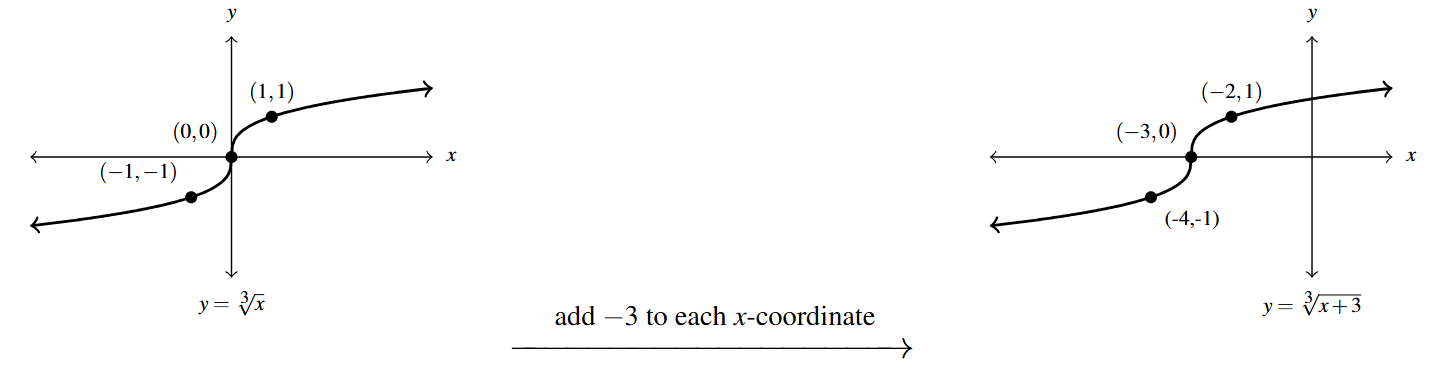
[latex]f(x) = -2 \sqrt[3]{x- (-3)} + 1[/latex]. We identify [latex]n=3[/latex], [latex]a = -2[/latex], [latex]b = 1[/latex], [latex]h = -3[/latex] and [latex]k = 1[/latex].
Step 1: add [latex]-3[/latex] to each of the [latex]x[/latex]-coordinates of each of the points on the graph of [latex]y=\sqrt[3]{x}[/latex]:
As [latex]b=1[/latex], we can proceed to Step 3 (dividing a real number by 1 results in the same real number.)
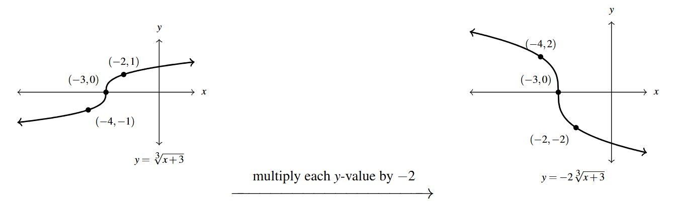
Step 3: multiply each of the [latex]y[/latex]-coordinates of each point on the graph of [latex]f_1 = \sqrt[3]{x+3}[/latex] by [latex]-2[/latex]:
Step 4: add 1 to [latex]y[/latex]-coordinates of each point on the graph of [latex]f_2 = -2 \sqrt[3]{x+3}[/latex]:
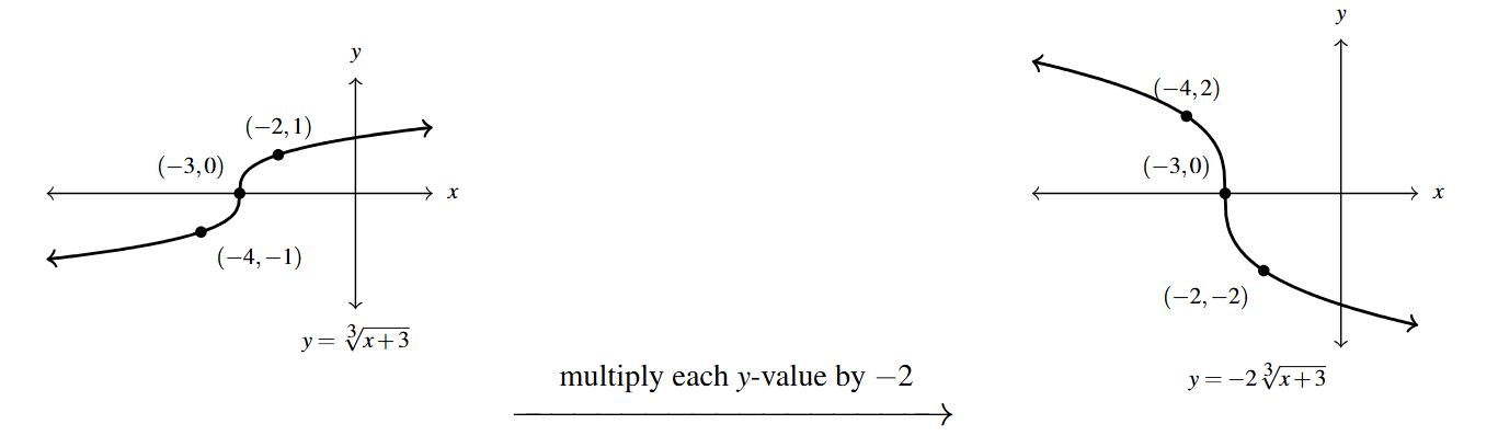
We get the domain and range of [latex]f[/latex] are both [latex](-\infty, \infty)[/latex].
Example 4.1.1.2
Use Theorem 4.1 to graph the following. Label at least three points and the asymptotes. State the domain and range using interval notation.
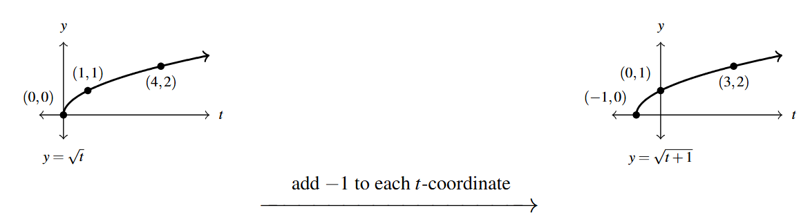
[latex]g(t) = \dfrac{\sqrt{1-2t}}{4}[/latex]
Solution:
Graph [latex]g(t) = \dfrac{\sqrt{1-2t}}{4}[/latex].
For [latex]g(t) = \dfrac{\sqrt{1-2t}}{4} = \dfrac{1}{4} \sqrt{-2t+1}[/latex], we identify [latex]n=2[/latex], [latex]a = \dfrac{1}{4}[/latex], [latex]b = -2[/latex], [latex]h = -1[/latex] and [latex]k =0[/latex].
We are asked to label three points on the graph, so we track [latex](4,2)[/latex] along with [latex](0,0)[/latex] and [latex](1,1)[/latex].[5]
Step 1: add [latex]-1[/latex] to each of the [latex]t[/latex]-coordinates of each of the points on the graph of [latex]y=\sqrt{t}[/latex]:
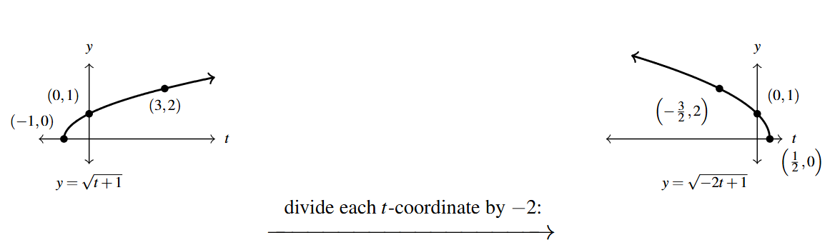
Step 2: divide each of the [latex]t[/latex]-coordinates of each of the points on the graph of [latex]g_1 = \sqrt{t+1}[/latex] by [latex]-2[/latex]:
Step 3: multiply each of the [latex]y[/latex]-coordinates of each of the points on the graph of [latex]g_2 = \sqrt{-2t+1}[/latex] by [latex]\dfrac{1}{4}[/latex]:
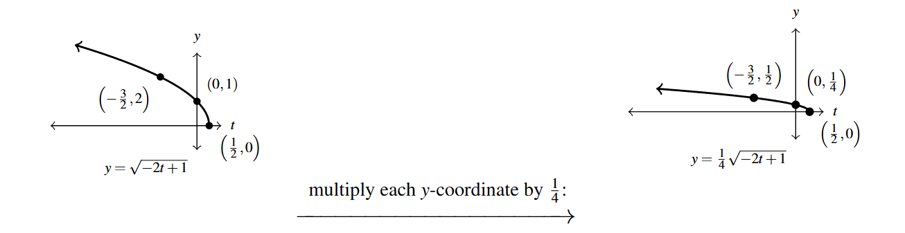
We get the domain is [latex]\left(-\infty, \dfrac{1}{2} \right][/latex] and the range is [latex][0, \infty)[/latex].
4.1.2 Other Functions involving Radicals
Now that we have some practice with basic root functions, we turn our attention to more general functions involving radicals. In general, Calculus is the best tool with which to study these functions. Nevertheless, we will use what algebra we know in combination with a graphing utility to help us visualize these functions and preview concepts which are studied in greater depth in later courses. In the table below, we summarize some of the properties of radicals from elsewhere in this text we will be using in the coming examples.
Suppose [latex]\sqrt[n]{x}[/latex], [latex]\sqrt[n]{a}[/latex], and [latex]\sqrt[n]{b}[/latex] are real numbers.[6]
Simplifying [latex]n[/latex]th powers and [latex]n[/latex]th roots:[7]
- [latex]\left( \sqrt[n]{x}\right)^n = x[/latex]
- if [latex]n[/latex] is odd, then [latex]\sqrt[n]{x^n} = x[/latex]
- if [latex]n[/latex] is even, then [latex]\sqrt[n]{x^n} = |x|[/latex]
Root Functions Preserve Inequality:[8] if [latex]a \leq b[/latex], then [latex]\sqrt[n]{a} \leq \sqrt[n]{b}[/latex]
Example 4.1.2
Example 4.1.2.1
For the following function: [latex]f(x) = 3x \sqrt[3]{2-x}[/latex]
- Analytically:
- State the domain
- Identify the axis intercepts
- Analyze the end behavior
- Construct a sign diagram for each function using the intercepts and sketch a graph
- Using technology determine:
- The range
- The local extrema, if they exist
- Intervals where the function is increasing
- Intervals where the function is decreasing
Solution:
Analyze and graph [latex]f(x) = 3x \sqrt[3]{2-x}[/latex].
When looking for the domain, we have two thing to watch out for: denominators (which we must make sure aren’t 0) and even indexed radicals (whose radicands we must ensure are nonnegative.)
Looking at the expression for [latex]f(x)[/latex], we have no denominators nor do we have an even indexed radical, so we are confident the domain is all real numbers, [latex](-\infty, \infty)[/latex].
As [latex](0,0)[/latex] is also on the [latex]y[/latex]-axis and functions can have at most one [latex]y[/latex]-intercept, we know [latex](0,0)[/latex] is the only [latex]y[/latex]-intercept.[9] That being said, we can quickly verify [latex]f(0) = 3(0) \sqrt[3]{2-0} = 0[/latex].
To determine the end behavior, we consider [latex]f(x)[/latex] as [latex]x \rightarrow \pm \infty[/latex]. Using number sense, [10] we have
\[ \begin{array}{rcl} f(x) &=& 3x \sqrt[3]{2-x} \\ &=& 3x \sqrt[3]{-x+2} \\ &\approx& (\text{big } (+)) \sqrt[3]{\text{big } (-)} \\ &=& (\text{big } (+))(\text{big } (-)) \\ &=& \text{big } (-) \end{array} \]
so [latex]f(x) \rightarrow -\infty[/latex].
As [latex]x \rightarrow -\infty[/latex] we get
\[ \begin{array}{rcl} f(x) &=& 3x \sqrt[3]{-x+2} \\ &\approx & (\text{big } (-)) \sqrt[3]{\text{big } (+)} \\ &=& (\text{big } (-))(\text{big } (+)) \\ &=& \text{big } (-) \end{array} \]
so [latex]f(x) \rightarrow -\infty[/latex] here, too.
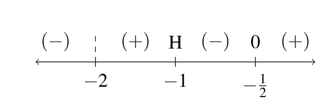
To create a sign diagram for [latex]f(x)[/latex], we note that the function has zeros [latex]x = 0[/latex] and [latex]x=2.[/latex]
For [latex]x[/latex] < 0, [latex]f(x)[/latex] < 0 or [latex](-)[/latex], for 0 < [latex]x[/latex] < 2, [latex]f(x) > 0[/latex] or [latex](+)[/latex], and for [latex]x>2[/latex], [latex]f(x)[/latex] < 0 or [latex](-).[/latex]
The sign diagram for [latex]f(x)[/latex] is below.
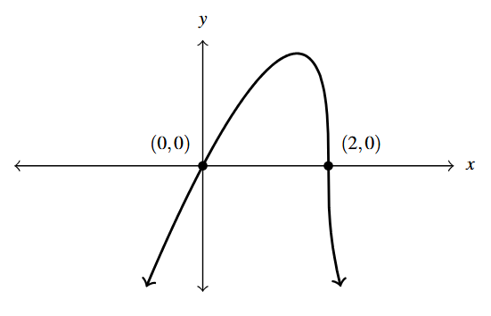
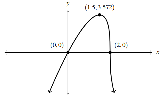
Putting all of the above together we get the graph of [latex]f[/latex]:
From the graph and our use of technology, the range is approximately [latex](-\infty, 3.572][/latex] with a local maximum (which also happens to be the maximum) at [latex](1.5, 3.572)[/latex]. We also see [latex]f[/latex] appears to be increasing on [latex](-\infty, 1.5)[/latex] and decreasing on [latex](1.5, \infty)[/latex].
It is also worth noting that there appears to be unusual steepness near the [latex]x[/latex]-intercept [latex](2,0)[/latex]. We invite the reader to zoom in on the graph near [latex](2,0)[/latex] to see that the function appears locally vertical.[11]
Example 4.1.2.2
For the following function: [latex]g(t) = \sqrt[3]{\dfrac{8t}{t+1}}[/latex]
- Analytically:
- State the domain
- Identify the axis intercepts
- Analyze the end behavior
- Construct a sign diagram for each function using the intercepts and sketch a graph
- Using technology determine:
- The range
- The local extrema, if they exist
- Intervals where the function is increasing
- Intervals where the function is decreasing
Solution:
Analyze and graph [latex]g(t) = \sqrt[3]{\dfrac{8t}{t+1}}[/latex].
The index of the radical in the expression for [latex]g(t)[/latex] is odd, so our only concern is the denominator. Setting [latex]t+1=0[/latex] gives [latex]t=-1[/latex], which we exclude, so our domain is [latex]\{ t \in \mathbb{R} \, | \, t \neq -1\}[/latex] or using interval notation, [latex](-\infty, -1) \cup (-1, \infty)[/latex].
If we take the time to analyze the behavior of [latex]g[/latex] near [latex]t=-1[/latex], we find that as [latex]t \rightarrow -1^{-},[/latex]
\[ \begin{array}{rcl} g(t) &=& \sqrt[3]{\dfrac{8t}{t+1}} \\ & & \\ &\approx & \sqrt[3]{\dfrac{-8}{\text{small } (-)}} \\ & & \\ &\approx & \sqrt[3]{\text{ big } (+)} \\ & & \\ &=& \text{big } (+) \end{array} \]
That is, as [latex]t \rightarrow -1^{-}[/latex], [latex]g(t) \rightarrow \infty[/latex].
Likewise, as [latex]t \rightarrow -1^{+},[/latex]
\[ \begin{array}{rcl} g(t) & \approx & \sqrt[3]{\dfrac{-8}{\text{small } (+)}} \\ & & \\ & \approx & \sqrt[3]{\text{ big } (-)} \\ & & \\ &=& \text{big } (-) \end{array} \]
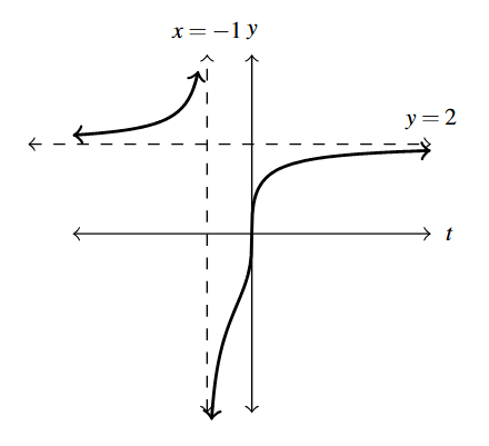
This suggests as [latex]t \rightarrow -1^{+}[/latex], [latex]g(t) \rightarrow -\infty[/latex]. This behavior points to a vertical asymptote, [latex]t=-1.[/latex]
To find the [latex]t[/latex]-intercepts of the graph of [latex]g[/latex], we find the zeros of [latex]g[/latex] by setting [latex]g(t) = \sqrt[3]{\dfrac{8t}{t+1}} = 0[/latex]. Cubing both sides and clearing denominators gives [latex]8t = 0[/latex] or [latex]t = 0[/latex]. Hence our [latex]t[/latex]-, and in this case, [latex]y[/latex]– intercept is [latex](0,0).[/latex]
To determine the end behavior, we note that as [latex]t \rightarrow \pm \infty ,[/latex]
\[ \dfrac{8t}{t+1} \rightarrow \dfrac{8}{1} = 8 \]
Hence, it stands to reason that as [latex]t\rightarrow \pm \infty ,[/latex]
\[ g(t) = \sqrt[3]{\dfrac{8t}{t+1}} \rightarrow \sqrt[3]{8} = 2\]
This suggests the graph of [latex]y = g(t)[/latex] has a horizontal asymptote at [latex]y = 2.[/latex]
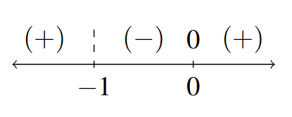
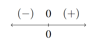
To create a sign diagram for [latex]g(t)[/latex], we note that the function is undefined when [latex]t = -1[/latex] (so we place a dashed line above it) and has a zero [latex]t=0.[/latex]
When [latex]t[/latex] < [latex]-1[/latex], [latex]g(t)[/latex] > 0 or [latex](+)[/latex], for [latex]-1[/latex] < [latex]t[/latex] < 0, [latex]g(t)[/latex] < 0 or [latex](-)[/latex], and for [latex]t>0[/latex], [latex]g(t) > 0[/latex] or [latex](+).[/latex]
A sign diagram for [latex]g(t)[/latex] is below.
The graph of [latex]f[/latex] is next.
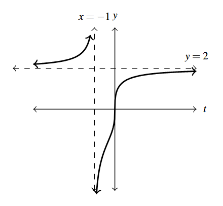
The graph confirms our suspicions about the asymptotes [latex]t = -1[/latex] and [latex]y = 2.[/latex]
Moreover, the range appears to be [latex](-\infty, 2) \cup (2, \infty)[/latex].
We could check if the graph ever crosses its horizontal asymptote by attempting to solve [latex]g(t) = \sqrt[3]{\dfrac{8t}{t+1}} = 2[/latex]. Cubing both sides and clearing denominators gives [latex]8t = 8(t+1)[/latex] which results in [latex]0 = 8[/latex], a contradiction. This proves 2 is not in the range, as we had suspected.
Scanning the graph, there appears to be no local extrema, and, moreover, the graph suggests [latex]g[/latex] is increasing on [latex](-\infty, -1)[/latex] and again on [latex](-1, \infty)[/latex]. As with the previous example, the graph appears locally vertical near its intercept [latex](0,0)[/latex].
Example 4.1.2.3
For the following function: [latex]h(x) = \dfrac{3x}{\sqrt{x^2 + 1}}[/latex]
- Analytically:
- State the domain
- Identify the axis intercepts
- Analyze the end behavior
- Construct a sign diagram for each function using the intercepts and sketch a graph
- Using technology determine:
- The range
- The local extrema, if they exist
- Intervals where the function is increasing
- Intervals where the function is decreasing
Solution:
Analyze and graph [latex]h(x) = \dfrac{3x}{\sqrt{x^2 + 1}}[/latex].
The expression for [latex]h(x) = \dfrac{3x}{\sqrt{x^2 + 1}}[/latex] has both a denominator and an even-indexed radical, so we have to be extra cautious here.
Fortunately for us, the quantity [latex]x^2+1 >0[/latex] for al real numbers [latex]x[/latex]. Not only does this mean [latex]\sqrt{x^2+1}[/latex] is always defined, it also tells us [latex]\sqrt{x^2+1}>0[/latex] for all [latex]x[/latex], too. This means the domain of [latex]h[/latex] is all real numbers, [latex](-\infty, \infty).[/latex]
Solving for the zeros of [latex]h[/latex] gives only [latex]x = 0[/latex], and we find, once again, [latex](0,0)[/latex] is both our lone [latex]x[/latex]– and [latex]y[/latex]-intercept.
Moving on to end behavior, as [latex]x \rightarrow \pm \infty[/latex], the term [latex]x^2[/latex] is the dominant term in the radicand in the denominator. As such,
\[ \begin{array}{rcl} h(x) &=& \dfrac{3x}{\sqrt{x^2 + 1}} \\ & & \\ & \approx & \dfrac{3x}{\sqrt{x^2}} \\ & & \\ &=& \dfrac{3x}{|x|} \end{array} \]
As [latex]x \rightarrow \infty[/latex], [latex]|x| = x[/latex] (because [latex]x>0[/latex]), so
\[h(x) \approx \dfrac{3x}{x} = 3,\]
so [latex]h(x) \rightarrow 3[/latex].
Likewise, as [latex]x \rightarrow -\infty[/latex], [latex]|x| = -x[/latex] (because [latex]x[/latex] < 0) and hence,
\[ h(x)\approx \dfrac{3x}{-x} = -3, \]
so [latex]h(x) \rightarrow -3[/latex].
This analysis suggests the graph of [latex]y=h(x)[/latex] has not one, but two horizontal asymptotes.[12] The graph of [latex]h[/latex] below bears this out.
The domain of [latex]h[/latex] is all real number and the only zero of [latex]h[/latex] is [latex]x=0[/latex], so the sign diagram for [latex]h(x)[/latex] is fairly straight forward. For [latex]x[/latex] < 0, [latex]h(x)[/latex] < 0 or [latex](-)[/latex] and for [latex]x>0[/latex], [latex]h(x) >0[/latex] or [latex](+).[/latex]
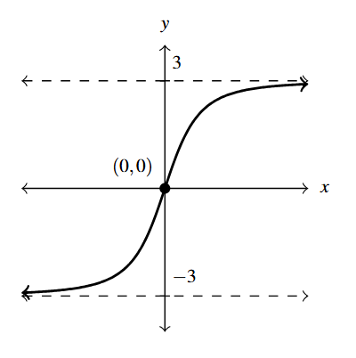
From the graph, we see the range of [latex]h[/latex] appears to be [latex](-3,3).[/latex]
Attempting to solve [latex]h(x) = \dfrac{3x}{\sqrt{x^2 + 1}} = \pm 3[/latex] gives, in either case, [latex]9x^2 = 9(x^2+1)[/latex] which reduces to [latex]0 = 9[/latex], a contradiction. Hence, the graph of [latex]y = h(x)[/latex] never reaches its horizontal asymptotes.
Moreover, [latex]h[/latex] appears to be always increasing, with no local extrema or unusual steepness.
One last remark: it appears as if the graph of [latex]h[/latex] is symmetric about the origin. We check [latex]h(-x) = \dfrac{3(-x)}{\sqrt{(-x)^2+1}} = - \dfrac{3x}{\sqrt{x^2 + 1}} = -h(x)[/latex] which verifies [latex]h[/latex] is odd.
Example 4.1.2.4
For the following function: [latex]r(t) = t^{-1} \sqrt{16t^4-1}[/latex]
- Analytically:
- State the domain
- Identify the axis intercepts
- Analyze the end behavior
- Construct a sign diagram for each function using the intercepts and sketch a graph
- Using technology determine:
- The range
- The local extrema, if they exist
- Intervals where the function is increasing
- Intervals where the function is decreasing
Solution:
Analyze and graph [latex]r(t) = t^{-1} \sqrt{16t^4-1}[/latex].
The first thing to note about the expression [latex]r(t) = t^{-1} \sqrt{16t^4-1}[/latex] is that [latex]t^{-1} = \dfrac{1}{t}[/latex].
Hence, we must exclude [latex]t=0[/latex] from the domain straight away.
Next, we have an even-indexed radical expression: [latex]\sqrt{16t^4-1}[/latex]. In order for this to return a real number, we require [latex]16t^4-1 \geq 0[/latex]. Instead of using a sign diagram to solve this, we opt instead to carefully use properties of radicals. Isolating [latex]t^4[/latex], we have [latex]t^4 \geq \dfrac{1}{16}[/latex]. As the root functions are increasing, we can apply the fourth root to both sides and preserve the inequality: [latex]\sqrt[4]{t^4} \geq \sqrt[4]{\dfrac{1}{16}}[/latex] which gives[13] [latex]|t| \geq \dfrac{1}{2}[/latex]. Note that [latex]t =0[/latex] does not satisfy this inequality, thus restricting [latex]t[/latex] in this manner takes care of both domain issues, so the domain is [latex]\left(-\infty, -\dfrac{1}{2} \right] \cup \left[\dfrac{1}{2}, \infty \right)[/latex].
Next, we look for zeros. Setting [latex]r(t) = t^{-1} \sqrt{16t^4-1} = \dfrac{\sqrt{16t^4-1}}{t}=0[/latex] gives [latex]\sqrt{16t^4-1} = 0[/latex]. After squaring both sides, we get [latex]16t^4-1 = 0[/latex] or [latex]t^4 = \dfrac{1}{16}[/latex]. Extracting fourth roots, we get [latex]t = \pm \dfrac{1}{2}[/latex]. Both of these are (barely!) in the domain of [latex]r[/latex], so our [latex]t[/latex] intercepts are [latex]\left( -\dfrac{1}{2}, 0\right)[/latex] and [latex]\left( \dfrac{1}{2}, 0\right).[/latex]
Note, the graph of [latex]r[/latex] has no [latex]y[/latex]-intercept, because [latex]r(0)[/latex] is undefined ([latex]t=0[/latex] is not in the domain of [latex]r[/latex]).
Concerning end behavior, we note the term [latex]16t^4[/latex] dominates the radicand [latex]\sqrt{16t^4-1}[/latex] as [latex]t \rightarrow \pm \infty[/latex], hence,
\[ \begin{array}{rcl} r(t) &=& \dfrac{\sqrt{16t^4-1}}{t} \\ & & \\ &\approx & \dfrac{\sqrt{16t^4}}{t} \\ & & \\ &=& \dfrac{4t^2}{t} \\ & & \\ &=& 4t \end{array} \]
This suggests the graph of [latex]y = r(t)[/latex] has a slant asymptote with slope 4.[14]
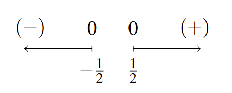
To construct the sign diagram for [latex]r(t)[/latex] we note [latex]r[/latex] has two zeros, [latex]t = \pm \dfrac{1}{2}[/latex].
For [latex]t[/latex] < [latex]\dfrac{1}{2}[/latex], [latex]r(t)[/latex] < 0 or [latex](-)[/latex] and when [latex]t > \dfrac{1}{2}[/latex], [latex]r(t) > 0[/latex] or [latex](+)[/latex]. When [latex]-\dfrac{1}{2}[/latex] < [latex]t[/latex] < [latex]\dfrac{1}{2}[/latex], [latex]r[/latex] is undefined so we have removed that segment from the diagram, as seen below.
The graph of [latex]r(t)[/latex]:
We see the range appears to be all real numbers, [latex](-\infty, \infty)[/latex].
It appears as if [latex]r[/latex] is increasing on [latex]\left(-\infty, -\dfrac{1}{2} \right)[/latex] and again on [latex]\left(\dfrac{1}{2}, \infty \right)[/latex].
The graph does appear to be asymptotic to [latex]y = 4t[/latex], and it also appears to be symmetric about the origin. Sure enough, we find [latex]r(-t) = \dfrac{\sqrt{16(-t)^4-1}}{-t} = - \dfrac{\sqrt{16t^4-1}}{t} = -r(t)[/latex], proving [latex]r[/latex] is an odd function.
We end this section with a classic application of root functions.
Example 4.1.3
Example 4.1.3.1
Carl wishes to get high speed internet service installed in his remote Sasquatch observation post located 30 miles from Route 117. The nearest junction box is located 50 miles down the road from the post, as indicated in the diagram below. Suppose it costs \$15 per mile to run cable along the road and \$20 per mile to run cable off of the road.
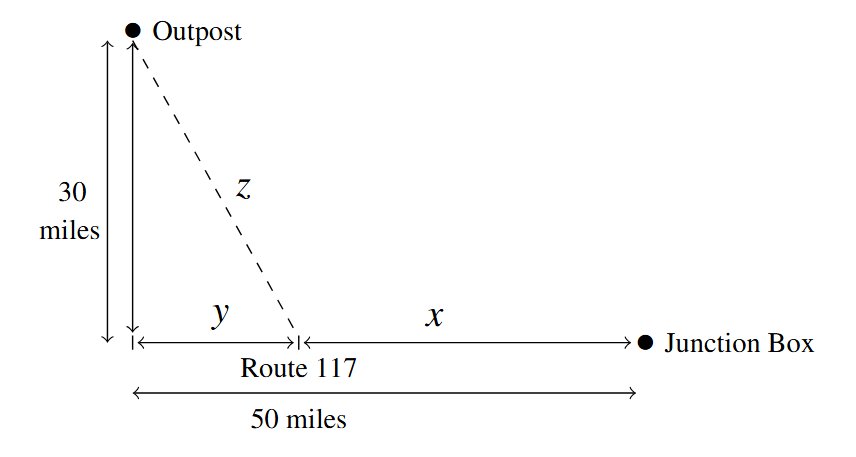
Write an expression, [latex]C(x)[/latex], which computes the cost of connecting the Junction Box to the Outpost as a function of [latex]x[/latex], the number of miles the cable is run along Route 117 before heading off road directly towards the Outpost. Determine a reasonable applied domain for the problem.
Solution:
Write an expression [latex]C(x)[/latex].
The cost is broken into two parts: the cost to run cable along Route 117 at \$15 per mile, and the cost to run it off road at \$20 per mile.
[latex]x[/latex] represents the miles of cable run along Route 117, thus the cost for that portion is [latex]15x[/latex].
From the diagram, we see that the number of miles the cable is run off road is [latex]z[/latex], so the cost of that portion is [latex]20z[/latex].
Hence, the total cost is [latex]15x + 20z[/latex].
Our next goal is to determine [latex]z[/latex] in terms of [latex]x[/latex]. The diagram suggests we can use the Pythagorean Theorem to get [latex]y^2+30^2 = z^2[/latex].
But we also see [latex]x+y = 50[/latex] so that [latex]y=50-x[/latex].
Substituting [latex](50-x)[/latex] in for [latex]y[/latex] we obtain [latex]z^2 = (50-x)^2+900[/latex].
Solving for [latex]z[/latex], we obtain [latex]z = \pm \sqrt{(50-x)^2+900}[/latex].
Because [latex]z[/latex] represents a distance, we choose [latex]z = \sqrt{(50-x)^2+900}[/latex].
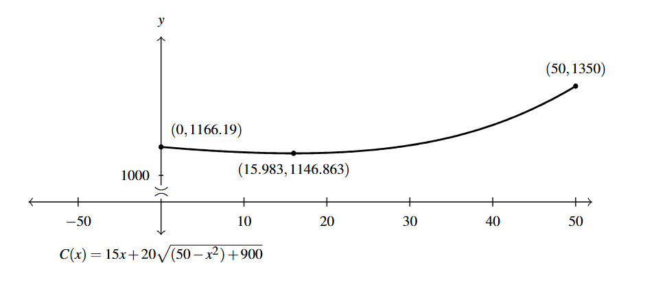
Hence, the cost as a function of [latex]x[/latex] is given by [latex]C(x) = 15x + 20\sqrt{(50-x)^2+900}[/latex]. From the context of the problem, we have [latex]0 \leq x \leq 50[/latex].
Example 4.1.3.2
Carl wishes to get high speed internet service installed in his remote Sasquatch observation post located 30 miles from Route 117. The nearest junction box is located 50 miles down the road from the post, as indicated in the diagram below. Suppose it costs \$ 15 per mile to run cable along the road and \$ 20 per mile to run cable off of the road.
Graph [latex]C(x)[/latex] on its domain. What is the minimum cost? How far along Route 117 should the cable be run before turning off of the road?
Solution:
Graph [latex]C(x)[/latex].
We graph [latex]y=C(x)[/latex] below and find our (local) minimum to be at the point [latex](15.98, 1146.86)[/latex], using technology.
Here the [latex]x[/latex]-coordinate tells us that in order to minimize cost, we should run 15.98 miles of cable along Route 117 and then turn off of the road and head towards the outpost. The [latex]y[/latex]-coordinate tells us that the minimum cost, in dollars, to do so is \$1146.86. The ability to stream live SasquatchCasts? Priceless.
4.1.3 Section Exercises
In Exercises 1 – 8, given the pair of functions [latex]f[/latex] and [latex]F[/latex], sketch the graph of [latex]y=F(x)[/latex] by starting with the graph of [latex]y = f(x)[/latex] and using Theorem 4.1. Track at least two points and state the domain and range using interval notation.
- [latex]f(x) = \sqrt{x}[/latex] and [latex]F(x) = \sqrt{x+3}-2[/latex]
- [latex]f(x) = \sqrt{x}[/latex] and [latex]F(x) = \sqrt{4-x}-1[/latex]
- [latex]f(x) = \sqrt[3]{x}[/latex] and [latex]F(x) = \sqrt[3]{x-1}-2[/latex]
- [latex]f(x) = \sqrt[3]{x}[/latex] and [latex]F(x) = -\sqrt[3]{8x + 8} + 4[/latex]
- [latex]f(x) = \sqrt[4]{x}[/latex] and [latex]F(x) = \sqrt[4]{x-1}-2[/latex]
- [latex]f(x) = \sqrt[4]{x}[/latex] and [latex]F(x) = -3\sqrt[4]{x - 7} +1[/latex]
- [latex]f(x) = \sqrt[5]{x}[/latex] and [latex]F(x) = \sqrt[5]{x + 2} + 3[/latex]
- [latex]f(x) = \sqrt[8]{x}[/latex] and [latex]F(x) = \sqrt[8]{-x} - 2[/latex]
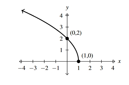
In Exercises 9 – 10, find a formula for each function below in the form [latex]F(x) = a\sqrt{bx-h}+k[/latex].
NOTE: There may be more than one solution!
- [latex]x-[/latex] and [latex]y-[/latex]intercept [latex](0,0)[/latex]
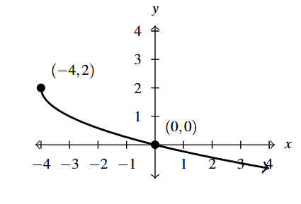
Graph for Exercise 9 - [latex]x-[/latex]intercept [latex](1,0)[/latex] and [latex]y-[/latex]intercept [latex](0,2)[/latex]
Graph for Exercise 10
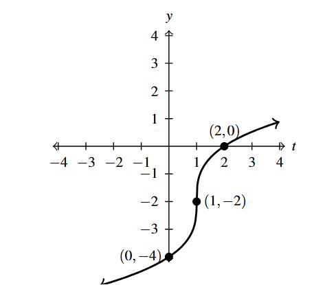
In Exercises 11 – 12, find a formula for each function below in the form [latex]F(x) = a\sqrt[3]{bx-h}+k[/latex].
NOTE: There may be more than one solution!
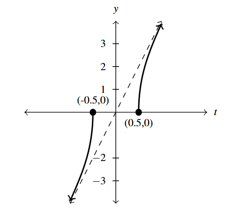
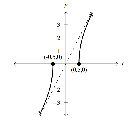
- [latex]x-[/latex]intercept [latex]\left( -\dfrac{1}{2},0 \right)[/latex] and [latex]y-[/latex]intercept [latex](0,-1)[/latex]
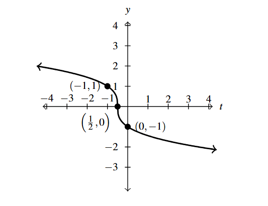
Graph for Exercise 11 - [latex]x-[/latex]intercept [latex](2,0)[/latex] and [latex]y-[/latex]intercept [latex](0,-4)[/latex]
Graph for Exercise 12 - Use the fact that the [latex]n[/latex]th root functions are increasing to solve the following polynomial inequalities:
- [latex]x^3 \leq 64[/latex]
- [latex]2 - t^5[/latex] < 34
- [latex]\dfrac{(2z+1)^3}{4} \geq 2[/latex]
For the following inequalities, remember [latex]\sqrt[n]{x^{n}} = |x|[/latex] if [latex]n[/latex] is even:
- [latex]x^4 \leq 16[/latex]
- [latex]6-t^6[/latex] < [latex]-58[/latex]
- [latex]\dfrac{(2z+1)^4}{3} \geq 27[/latex]
For each function in Exercises 14 – 21 below
- Analytically:
- State the domain
- Determine the axis intercepts
- Analyze the end behavior
- Construct a sign diagram for each function using the intercepts and sketch a graph.
- Using technology determine:
- The range
- The local extrema, if they exist
- Intervals where the function is increasing/decreasing
- Any unusual steepness or local verticality
- Vertical asymptotes
- Horizontal/slant asymptotes
- Comment on any observed symmetry
- [latex]f(x) = \sqrt{1 - x^{2}}[/latex]
- [latex]f(x) = \sqrt{x^2-1}[/latex]
- [latex]g(t) = t \sqrt{1-t^2}[/latex]
- [latex]g(t) = t \sqrt{t^2-1}[/latex]
- [latex]f(x) = \sqrt[4]{\dfrac{16x}{x^{2} - 9}}[/latex]
- [latex]f(x) = \dfrac{5x}{\sqrt[3]{x^{3} + 8}}[/latex]
- [latex]g(t) = \sqrt{t(t + 5)(t - 4)}[/latex]
- [latex]g(t) = \sqrt[3]{t^{3} + 3t^{2} - 6t - 8}[/latex]
- Rework Example 4.1.3 so that the outpost is 10 miles from Route 117 and the nearest junction box is 30 miles down the road for the post.
- The volume [latex]V[/latex] of a right cylindrical cone depends on the radius of its base [latex]r[/latex] and its height [latex]h[/latex] and is given by the formula [latex]V = \dfrac{1}{3} \pi r^2 h[/latex]. The surface area [latex]S[/latex] of a right cylindrical cone also depends on [latex]r[/latex] and [latex]h[/latex] according to the formula [latex]S = \pi r \sqrt{r^2+h^2}[/latex]. In the following problems, suppose a cone is to have a volume of 100 cubic centimeters.
- Use the formula for volume to find the height as a function of [latex]r[/latex], [latex]h(r)[/latex].
- Use the formula for surface area along with your answer to 23a to find the surface area as a function of [latex]r[/latex], [latex]S(r)[/latex].
- Use your calculator to find the values of [latex]r[/latex] and [latex]h[/latex] which minimize the surface area. What is the minimum surface area? Round your answers to two decimal places.
- The period of a pendulum in seconds is given by \[T = 2\pi \sqrt{\dfrac{L}{g}}\](for small displacements) where [latex]L[/latex] is the length of the pendulum in meters and [latex]g = 9.8[/latex] meters per second per second is the acceleration due to gravity. My Seth-Thomas antique schoolhouse clock needs [latex]T = \dfrac{1}{2}[/latex] second and I can adjust the length of the pendulum via a small dial on the bottom of the bob. At what length should I set the pendulum?
- According to Einstein’s Theory of Special Relativity, the observed mass of an object is a function of how fast the object is traveling. Specifically, if [latex]m_{r}[/latex] is the mass of the object at rest, [latex]v[/latex] is the speed of the object and [latex]c[/latex] is the speed of light, then the observed mass of the object [latex]m(v)[/latex] is given by:\[m(v) = \dfrac{m_{r}}{\sqrt{1 – \dfrac{v^{2}}{c^{2}}}}\]
- State the applied domain of the function.
- Compute [latex]m(.1c), \, m(.5c), \, m(.9c)[/latex] and [latex]m(.999c)[/latex].
- As [latex]v \rightarrow c^{-}[/latex], what happens to [latex]m(x)[/latex]?
- How slowly must the object be traveling so that the observed mass is no greater than 100 times its mass at rest?
- Find the inverse of [latex]k(x) = \dfrac{2x}{\sqrt{x^{2} - 1}}[/latex].
Section 4.1 Exercise Answers can be found in the Appendix.
- Although we discussed imaginary numbers in Section 1.5, we restrict our attention to real numbers in this section. ↵
- See Exercise 13. ↵
- Because, otherwise, [latex]-1 = i^2 = i \cdot i = \sqrt{-1}\sqrt{-1} = \sqrt{(-1)(-1)} = \sqrt{1} = 1[/latex], a contradiction. ↵
- again this is because every real number can be represented as both [latex]x-h[/latex] for some value [latex]x[/latex] and as [latex]c+h[/latex] for some value [latex]c[/latex]. ↵
- As [latex]\sqrt{4} = 2[/latex], we know [latex](4,2)[/latex] is on the graph of [latex]y = \sqrt{t}[/latex]. ↵
- i.e., if [latex]n[/latex] is odd, [latex]x[/latex], [latex]a[/latex], and [latex]b[/latex] can be any real numbers; if, on the other hand [latex]n[/latex] is even, [latex]x \geq 0[/latex], [latex]a \geq 0[/latex], and [latex]b \geq 0[/latex]. ↵
- a.k.a., Inverse Properties. See Section 5.1. ↵
- i.e., root functions are increasing. ↵
- Why is this, again? ↵
- remember this means we use the adjective big here to mean large in absolute value ↵
- Of course, the Vertical Line Test prohibits the graph from actually being a vertical line. This behavior is more precisely defined and more closely studied in Calculus. ↵
- We warned you this was coming [latex]\ldots[/latex] see the discussion following Theorem 3.3 in Section 3.2. ↵
- Recall: [latex]\sqrt[n]{x^n} = |x|[/latex], not [latex]x[/latex], if [latex]n[/latex] is even. ↵
- Note: this analysis suggests the slant asymptote is [latex]y = 4t+b[/latex], but from this analysis, we cannot determine the value of [latex]b[/latex]. As with slant asymptotes in Section 3.2, we'd need to perform a more detailed analysis which we omit in this case owing to the complexity of the function. ↵
