
9.1 Vectors
As we have seen numerous times in this book, Mathematics can be used to model and solve real-world problems. For many applications, real numbers suffice; that is, real numbers with the appropriate units attached can be used to answer questions like “How close is the nearest Sasquatch nest?”
There are other times though, when these kinds of quantities do not suffice. Perhaps it is important to know, for instance, how close the nearest Sasquatch nest is as well as the direction in which it lies. To answer questions like these which involve both a quantitative answer, or magnitude, along with a direction, we use the mathematical objects called vector.[1]
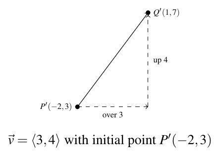
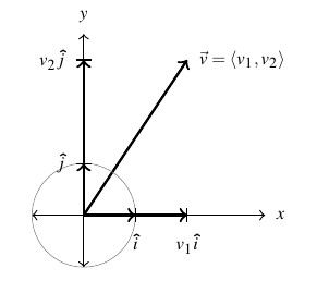
A vector is represented geometrically as a directed line segment where the magnitude of the vector is taken to be the length of the line segment and the direction is made clear with the use of an arrow at one endpoint of the segment. When referring to vectors in this text, we shall adopt[2] the `arrow’ notation, so the symbol  is read as `the vector
  ‘. Below is a typical vector with endpoints
  and
and  .
.
The point  is called the tail of and the point
  is called the terminal point or head of . We can reconstruct completely from and , so we write
  , where the order of points (initial point) and (terminal point) is important. (Think about this before moving on.)

While it is true that and completely determine , it is important to note that because vectors are defined in terms of their two characteristics, magnitude and direction, any directed line segment with the same length and direction as is considered to be the same vector as , regardless of its initial point.
In the case of our vector above, any vector which moves three units to the right and four up[3] from its initial point to arrive at its terminal point is considered the same vector as . The notation we use to capture this idea is the component form of the vector,  , where the first number,
  , is called the
  –component of and the second number,
  , is called the
  –component of .
For example, if we wanted to reconstruct with initial point  , then we would find the terminal point of by adding to the -coordinate and adding to the -coordinate to obtain the terminal point
  .
.
The component form of a vector is what ties these very geometric objects back to Algebra and ultimately Trigonometry. We generalize our example in our definition below.
Definition 9.1
Suppose is represented by a directed line segment with initial point  and terminal point
  . The component form of is given by
![\[ \vec{v} = \overrightarrow{PQ} = \left< x_{1} - x_{0}, y_{1} - y_{0} \right> \]](https://odp.library.tamu.edu/app/uploads/quicklatex/quicklatex.com-325797e209f55da75b44f83f50608206_l3.png "Rendered by QuickLaTeX.com")
Using the language of components, we have that two vectors are equal if and only if their corresponding components are equal. That is,  if and only if
  and
and  . (Again, think about this before reading on.)
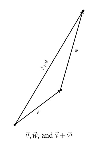
We now set about defining operations on vectors. Suppose we are given two vectors and  . The sum, or resultant vector
  is obtained as follows. First, plot . Next, plot so that its initial point is the terminal point of . To plot the vector we begin at the initial point of and end at the terminal point of . It is helpful to think of the vector as the `net result’ of moving along then moving along .
Our next example makes good use of resultant vectors and reviews bearings and the Law of Cosines.[4]
Example 9.1.1
Example 9.1.1
A plane leaves an airport with an airspeed[5] of 175 miles per hour at a bearing of N E. A 35 mile per hour wind is blowing at a bearing of S
 E. Find the true speed of the plane, rounded to the nearest mile per hour, and the true bearing of the plane, rounded to the nearest degree.
Solution:
For both the plane and the wind, we are given their speeds and their directions. Coupling speed (as a magnitude) with direction is the concept of velocity which we’ve seen a few times before.[6]
We let denote the plane’s velocity and denote the wind’s velocity in the diagram below. The `true’ speed and bearing is found by analyzing the resultant vector, .
From the vector diagram, we get a triangle, the lengths of whose sides are the magnitude of , which is 175, the magnitude of , which is 35, and the magnitude of , which we’ll call  .
.
From the given bearing information, we go through the usual geometry to determine that the angle between the sides of length 35 and 175 measures  .
.

From the Law of Cosines, we determine  , which means the true speed of the plane is (approximately)
  miles per hour.
To determine the true bearing of the plane, we need to determine the angle  . Using the Law of Cosines once more,[7] we find
  so that
  .
.
Given the geometry of the situation, we add to the given and find the true bearing of the plane to be (approximately) N E.
E.
Our next step is to define addition of vectors component-wise to match the geometric action.[8]
![\[ \vec{v} + \vec{w} = \left< v_{1} + w_{1}}, v_{2} + w_{2} \right> \]](https://odp.library.tamu.edu/app/uploads/quicklatex/quicklatex.com-9aea773dbadab7b7cfba4c454fd420b8_l3.png "Rendered by QuickLaTeX.com")
Example 9.1.2
Example 9.1.2
Let and suppose  where
where  and
and  . Compute and interpret this sum geometrically.
Solution:
Before we can add the vectors using Definition 9.2, we need to write in component form. Using Definition 9.1, we get  . Thus,
![\[\vec{v} + \vec{w} = \left<3,4\right> + \left<1,-2\right> = \left< 3 + 1, 4 + (-2) \right> = \left<4, 2\right>. \]](https://odp.library.tamu.edu/app/uploads/quicklatex/quicklatex.com-6a4f46a930e623bfdac133908a500342_l3.png "Rendered by QuickLaTeX.com")
To visualize this sum, we draw with its initial point at  (for convenience) so that its terminal point is
  . Next, we graph with its initial point at . Moving one to the right and two down, we find the terminal point of to be
  .
.

We see the vector has initial point and terminal point so its component form is 
In order for vector addition to enjoy the same kinds of properties as real number addition, it is necessary to extend our definition of vectors to include a `zero vector’, 
Geometrically,  represents a point, which we can (very broadly) think of as a directed line segment with the same initial and terminal points. The reader may well object to the inclusion of , because after all, vectors are supposed to have both a magnitude (length) and a direction.
While it seems clear that the magnitude of should be  , it is not clear what its direction is. As we shall see, the direction of is in fact undefined, but this minor hiccup in the natural flow of things is worth the benefits we reap by including in our discussions. We have the following theorem.
Theorem 9.1 Properties of Vector Addition
- Commutative Property: For all vectors
 ,
, 
- Associative Property: For all vectors
 ,
, 
- Identity Property: For all vectors ,
![\[\vec{v} + \vec{0} = \vec{0} + \vec{v} = \vec{v}.\]](https://odp.library.tamu.edu/app/uploads/quicklatex/quicklatex.com-2b5cbc27acb161aa24de1ccd3dbdfe1a_l3.png "Rendered by QuickLaTeX.com")
The vector
acts as the additive identity for vector addition. - Inverse Property: For every vector
 , the vector
  satisfies
![\[\vec{v} + \vec{w} = \vec{w} + \vec{v} = \vec{0}.\]](https://odp.library.tamu.edu/app/uploads/quicklatex/quicklatex.com-cf1692a8bfa21dd8aba9c0b43507b386_l3.png "Rendered by QuickLaTeX.com")
That is, the additive inverse of a vector is the vector of the additive inverses of its components.
The properties in Theorem 9.1 are easily verified using the definition of vector addition, and are a direct consequence of the definition of vector addition along with properties inherited from real number arithmetic.
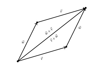
For the commutative property, we note that if  and
and  then
then
![\[ \begin{array}{rcl} \vec{v} + \vec{w} & = & \left< v_{1}, v_{2} \right> + \left< w_{1}, w_{2} \right> \\ & = & \left< v_{1} + w_{1}, v_{2} + w_{2} \right> \\ & = & \left< w_{1} + v_{1}, w_{2} + v_{2} \right> \\ & = & \vec{w} + \vec{v} \end{array} \]](https://odp.library.tamu.edu/app/uploads/quicklatex/quicklatex.com-43e734e77ef31172c6645007abc62fea_l3.png "Rendered by QuickLaTeX.com")
Geometrically, we can `see’ the commutative property by realizing that the sums  and
and  are the same directed diagonal determined by the parallelogram below.
The proofs of the associative and identity properties proceed similarly, and the reader is encouraged to verify them and provide accompanying diagrams.
The additive identity property is likewise verified algebraically using a calculation. If , then
![\[ \begin{array}{rcl} \vec{v} + \vec{0} &=& \left<v_{1},v_{2}\right> + \left<0, 0\right>\\ &=& \left< v_{1} + 0, v_{2} + 0 \right>\\ &=& \left<v_{1},v_{2}\right>\\ &=& \vec{v} \end{array}\]](https://odp.library.tamu.edu/app/uploads/quicklatex/quicklatex.com-62756a935677ca345a71e1ec10cba3fb_l3.png "Rendered by QuickLaTeX.com")
From the commutative property of vector addition, we get that  as well. Again, the reader is encouraged to visualize what this means geometrically.[9]
Regarding additive inverses, we can verify by direct computation that if and ,
![\[ \begin{array}{rcl} \vec{v} + \vec{w} &=& \left< v_{1}, v_{2} \right> + \left< - v_{1}, -v_{2} \right> \\ &=& \left< v_{1} + ( - v_{1}), v_{2} + ( - v_{2}) \right> \\ &=& \left< 0,0 \right> \\ &=& \vec{0} \end{array}\]](https://odp.library.tamu.edu/app/uploads/quicklatex/quicklatex.com-742f283065180b4e6b0c1523f9aee4c6_l3.png "Rendered by QuickLaTeX.com")
Once again, the commutative property of vector addition assures us that, likewise, 
Moreover, additive inverses of vectors are unique. That is, given a vector  , there is precisely only one vector so that
To see this, suppose a vector satisfies  . By the definition of vector addition, we have
  . Hence,
  and
and  . We get
  and
and  so that
  as prescribed in Theorem 9.1.
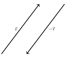
Hence, every vector has one, and only one, additive inverse. In general, we denote the additive inverse of a vector with the (highly suggestive) notation 
Geometrically, the vectors and  have the same length, but opposite directions. As a result, when adding the vectors geometrically, the sum
  results in starting at the initial point of and ending back at the initial point of . That is, the net result of moving then
  is not moving at all.
Using the additive inverse of a vector, we can define the difference of two vectors:  . Looking at this at the level of components, we see if and then
![\[\begin{array}{rcl} \vec{v} - \vec{w} & = & \vec{v} + (-\vec{w}) \\ & = & \left<v_{1},v_{2}\right> + \left<-w_{1},-w_{2}\right> \\ & = & \left<v_{1} + \left(-w_{1}\right),v_{2} + \left(-w_{2}\right) \right>\\ & = & \left<v_{1} -w_{1},v_{2} - w_{2}\right> \\ \end{array} \]](https://odp.library.tamu.edu/app/uploads/quicklatex/quicklatex.com-9b6535b802daf3f9141cf46e2afbf25b_l3.png "Rendered by QuickLaTeX.com")
In other words, like vector addition, vector subtraction works component-wise.
To interpret the vector  geometrically, we note
![\[ \begin{array}{rcll} \vec{w} + \left(\vec{v} - \vec{w}\right) & = & \vec{w} + \left(\vec{v} +(-\vec{w})\right) & \text{Definition of Vector Subtraction} \\ & = & \vec{w} + \left((-\vec{w})+\vec{v}\right) & \text{Commutativity of Vector Addition} \\ & = & (\vec{w} + (-\vec{w})) + \vec{v} & \text{Associativity of Vector Addition} \\ & = & \vec{0} + \vec{v} & \text{Definition of Additive Inverse}\\ & = & \vec{v} & \text{Definition of Additive Identity} \\ \end{array} \]](https://odp.library.tamu.edu/app/uploads/quicklatex/quicklatex.com-97d6645c909a82c3052c54ac63c615bf_l3.png "Rendered by QuickLaTeX.com")
This means that the `net result’ of moving along then moving along is just itself.
From the diagram below on the left, we see that  may be interpreted as the vector whose initial point is the terminal point of and whose terminal point is the terminal point of
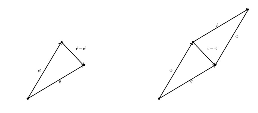
It is also worth mentioning that in the parallelogram determined by the vectors and above on the right, the vector is one of the diagonals — the other being .
Next, we discuss scalar multiplication — that is, taking a real number times a vector.
 by
by ![\[k\vec{v} = k\left<v_{1},v_{2}\right> =\left<k v_{1},k v_{2}\right> \]](https://odp.library.tamu.edu/app/uploads/quicklatex/quicklatex.com-5ccadd61f6948a9eab779d81d653ee7a_l3.png "Rendered by QuickLaTeX.com")
Scalar multiplication by  in vectors can be understood geometrically as scaling the vector (if
  ) or scaling the vector and reversing its direction (if
  ) as demonstrated below.
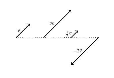
Note by Definition 9.3,  , which is what we would expect. This and other properties of scalar multiplication are summarized in the next theorem.
Theorem 9.2 Properties of Scalar Multiplication
- Associative Property: For every vector and scalars and
 ,
, 
- Identity Property: For all vectors ,

- Additive Inverse Property: For all vectors ,
 .
. - Distributive Property of Scalar Multiplication over Scalar Addition: For every vector and scalars and ,
![\[(k+r)\vec{v} = k\vec{v} + r\vec{v}\]](https://odp.library.tamu.edu/app/uploads/quicklatex/quicklatex.com-f71b077a7a96d81fe3567c4745156f6e_l3.png "Rendered by QuickLaTeX.com")
- Distributive Property of Scalar Multiplication over Vector Addition: For all vectors and and scalars ,
![\[k(\vec{v}+\vec{w}) = k\vec{v} + k\vec{w}\]](https://odp.library.tamu.edu/app/uploads/quicklatex/quicklatex.com-69f55a8a1916c48225b5bd8f0dc9f7a7_l3.png "Rendered by QuickLaTeX.com")
- Zero Product Property: If is vector and is a scalar, then
![\[k\vec{v} = \vec{0} \quad \text{if and only if} \quad k=0 \quad \text{or} \quad \vec{v} =\vec{0}\]](https://odp.library.tamu.edu/app/uploads/quicklatex/quicklatex.com-6cabc37f49524b4deca55388c98677d7_l3.png "Rendered by QuickLaTeX.com")
The proof of Theorem 9.2, like the proof of Theorem 9.1, ultimately boils down to the definition of scalar multiplication and properties of real numbers.
For example, to prove the associative property, we let . If and are scalars then
![\[\begin{array}{rcll} (kr) \vec{v} & = & (kr) \left<v_{1},v_{2}\right> & \\ [3pt] & = & \left<(kr) v_{1}, (kr) v_{2}\right> & \text{Definition of Scalar Multiplication} \\ [3pt] & = &\left<k (r v_{1}), k (r v_{2})\right> & \text{Associative Property of Real Number Multiplication} \\ [3pt] & = & k\left<r v_{1}, r v_{2}\right> & \text{Definition of Scalar Multiplication} \\ [3pt] & = & k\left(r\left<v_{1}, v_{2}\right>\right) & \text{Definition of Scalar Multiplication} \\ [3pt] & = & k(r\vec{v}) & \\ \end{array} \]](https://odp.library.tamu.edu/app/uploads/quicklatex/quicklatex.com-91a6599721a17f6e7af428d08c5d212c_l3.png "Rendered by QuickLaTeX.com")
The reader is invited to think about what this property means geometrically. The remaining properties are proved similarly and are left as exercises.
Our next example demonstrates how Theorem 9.2 allows us to do the same kind of algebraic manipulations with vectors as we do with variables — multiplication and division of vectors notwithstanding. If the pedantry seems familiar, it should.
Example 9.1.3
Example 9.1.3
Solve  for
for
Solution:
![\[ \begin{array}{rcl} 5\vec{v} - 2\left(\vec{v} +\ \left<1,-2\right>\right) & = & \vec{0} \\ 5\vec{v} + (-1)\left[ 2\left(\vec{v} +\left<1,-2\right>\right)\right] & = & \vec{0}\\ 5\vec{v} + [(-1)(2)]\left(\vec{v} + \left<1,-2\right>\right) & = & \vec{0}\\ 5\vec{v} + (-2)\left(\vec{v} + \left<1,-2\right>\right) & = & \vec{0}\\ 5\vec{v} + \left[(-2)\vec{v} + (-2)\left<1,-2\right> \right] & = & \vec{0}\\ 5\vec{v} + \left[(-2)\vec{v} + \left<(-2)(1),(-2)(-2)\right> \right] & = & \vec{0}\\ \left[5\vec{v} + (-2)\vec{v}\right] + \left<-2,4\right> & = & \vec{0}\\ (5 + (-2)) \vec{v} + \left<-2,4\right> & = & \vec{0}\\ 3\vec{v} + \left<-2,4\right> & = & \vec{0}\\ \left(3\vec{v} + \left<-2,4\right>\right) + \left(- \left<-2,4\right>\right) & = & \vec{0} + \left(- \left<-2,4\right>\right)\\ 3\vec{v} + \left[\left<-2,4\right> + \left(- \left<-2,4\right>\right)\right] & = & \vec{0} + (-1) \left<-2,4\right>\\ 3\vec{v} + \vec{0} & = & \vec{0} + \left<(-1)(-2),(-1)(4)\right>\\ 3\vec{v} & = & \left<2,-4\right>\\[3pt] \frac{1}{3} \left(3\vec{v} \right) & = & \frac{1}{3} \left(\left<2,-4\right>\right)\\[3pt] \left[\left(\frac{1}{3}\right) (3) \right]\vec{v} & = & \left< \left(\frac{1}{3}\right)(2), \left(\frac{1}{3}\right)(-4)\right>\\[3pt] 1 \vec{v} & = & \left< \frac{2}{3}, -\frac{4}{3} \right> \\[3pt] \vec{v} & =& \left< \frac{2}{3}, -\frac{4}{3} \right> \\ \end{array} \]](https://odp.library.tamu.edu/app/uploads/quicklatex/quicklatex.com-fc424f6337173b18e245b9eeffb483de_l3.png "Rendered by QuickLaTeX.com")
The reader is invited to check our solution in the original equation.
A vector whose initial point is is said to be in standard position. If is plotted in standard position, then its terminal point is necessarily  . (Once more, think about this before reading on.)
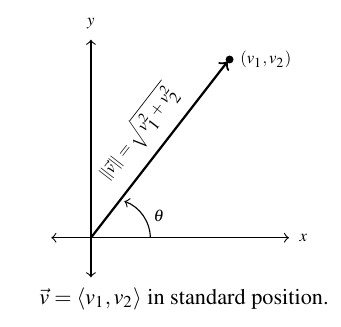
Plotting a vector in standard position enables us to more easily quantify the concepts of magnitude and direction of the vector.
Recall the magnitude of vector is the length of the directed line segment representing . When plotted in standard position, the length of this line segment is none other than the distance from the origin to the point . Hence, the magnitude of , which we denote  , is given by
Turning to the notion of direction, we note that the point is on the terminal side of the angle  depicted in the diagram above. From Theorem 7,4, we have
  and
and  . From the definition of scalar multiplication and vector equality, we get
![\[ \begin{array}{rcl} \vec{v} & = & \left< v_{1} , v_{2} \right> \\ [3pt] & = & \left< \| \vec{v} \| \cos(\theta), \| \vec{v} \| \sin(\theta) \right> \\ [3pt] & = & \| \vec{v} \| \left< \cos(\theta),\sin(\theta) \right> \\ \end{array} \]](https://odp.library.tamu.edu/app/uploads/quicklatex/quicklatex.com-8e03bcf0a8ac0fbd89feed0c4f3c5f73_l3.png "Rendered by QuickLaTeX.com")
This motivates the following definition.
Definition 9.4
Suppose is a vector with component form  .
.
- The magnitude of , denoted , is given by

- The direction angle of , denoted , is given by

Note: is an angle in standard position whose terminal side contains the point . - If
 , directional vector of , denoted
  is given by
Taken together, we get  .
.
A few remarks are in order. First, we note that if  then there are infinitely many angles which satisfy Definition 9.4. However, the fact that all of them must contain the same point on their terminal sides means they are all coterminal.
Hence, if and  both satisfy the conditions of Definition 9.4, then
  and
and  , and as such,
  making is well-defined.
For  , note that
  . Hence,
  for every angle . In other words, every angle satisfies the equation in Definition 9.4, so for this reason,
  is undefined.
The following theorem summarizes the important facts about the magnitude and direction of a vector.
Theorem 9.3 Properties of Magnitude and Direction
Suppose is a vector.
 and
and  if and only if
- For all scalars ,

- If then
 , so that
  . [10]
The proof of the first property in Theorem 9.3 is a direct consequence of the definition of . Given  , then which is by definition greater than or equal to . Moreover,
  if and only of
  if and only if
  . Hence, if and only if
  , as required.
The second property is a result of the definition of magnitude and scalar multiplication along with a property of radicals. If and is a scalar then
![\[ \begin{array}{rcll} \| k \, \vec{v} \| & = & \| k \left< v_{1}, v_{2}\right> \| & \\ [3pt]& = & \| \left<kv_{1},kv_{2}\right>\| & \text{Definition of scalar multiplication} \\ [3pt]& = & \sqrt{\left(kv_{1}\right)^2 + \left(kv_{2}\right)^2} & \text{Definition of magnitude} \\ [3pt]& = & \sqrt{k^2v_{1}^2 + k^2v_{2}^2} & \\[3pt]& = & \sqrt{k^2(v_{1}^2+v_{2}^2)} & \\ [3pt] & = & \sqrt{k^2} \sqrt{v_{1}^2+v_{2}^2} & \text{Product Rule for Radicals} \\ [3pt]& = & |k| \sqrt{v_{1}^2+v_{2}^2} & \text{$\sqrt{k^2} = |k|$} \\& = & |k| \| \vec{v} \| & \\ \end{array} \]](https://odp.library.tamu.edu/app/uploads/quicklatex/quicklatex.com-3143a5a0ad8d0b72487e8f732a78778a_l3.png "Rendered by QuickLaTeX.com")
The equation in Theorem 9.3 is a consequence of the definitions of and and was worked out in the discussion just prior to Definition 9.4. In words, the equation says that any given vector is the product of its magnitude and its direction — an important concept to keep in mind when studying and using vectors.
The formula for stated in Theorem 9.3 is a consequence of solving for by multiplying[11] both sides of the equation by  and using the properties of Theorem 9.2. We leave these details to the reader. We are overdue for an example.
Example 9.1.4
Example 9.1.4.1
Write the component form of the vector with  so that when is plotted in standard position, it lies in Quadrant II and makes a angle[12] with the negative -axis.
Solution:
Write the component form of the vector with so that when is plotted in standard position, it lies in Quadrant II and makes a angle with the negative -axis.
We are told that  and are given information about its direction, so we can use the formula to get the component form of
To determine , we appeal to Definition 9.4. Because lies in Quadrant II and makes a angle with the negative -axis, one angle satisfying the criteria of Definition 9.4 is 

Hence,
![\[ \begin{array}{rcl} \bm\hat{v} &=& \left< \cos\left(120^{\circ}\right), \sin\left(120^{\circ}\right) \right>\\[10pt] &=& \left< - \frac{1}{2} , \frac{\sqrt{3}}{2} \right> \end{array} \]](https://odp.library.tamu.edu/app/uploads/quicklatex/quicklatex.com-cbcaa0f8175a30b2940d95bf95d06aa3_l3.png "Rendered by QuickLaTeX.com")
so the result is
![\[ \begin{array}{rcl} \vec{v} &=& \| \vec{v} \| \bm\hat{v}\\ &=& 5 \left< - \frac{1}{2} , \frac{\sqrt{3}}{2} \right>\\[10pt] &=& \left< - \frac{5}{2} , \frac{5\sqrt{3}}{2} \right> \end{array} \]](https://odp.library.tamu.edu/app/uploads/quicklatex/quicklatex.com-0e44a1716ddc1b696f0166c74d7f840c_l3.png "Rendered by QuickLaTeX.com")
Example 9.1.4.2
For  , compute
  and ,
and ,  so that
  .
.
Solution:
For , compute and , so that 
For , we get  .
.
In light of Definition 9.4, we can find the we’re after by finding a Quadrant IV angle whose terminal side contains the point  .
.
We compute using the definition of the direction angle of , 
![\[ \begin{array}{lcl} \theta & = & \arctan \left( \dfrac{v_{2}}{v_{1}} \right) \\[4pt] & = & \arctan \left( \dfrac{-3\sqrt{3}}{3} \right) \\[4pt] & = & \arctan \left( - \sqrt{3} \right) \\[4pt] & = & - \frac{\pi}{3} + \pi k, \text{ where } k \text{ is any integer} \\ \end{array}\]](https://odp.library.tamu.edu/app/uploads/quicklatex/quicklatex.com-e5cf205ac9155808672b0880789a0c04_l3.png "Rendered by QuickLaTeX.com")
As the terminal side of is in Quadrant IV, we let  resulting in
We may check our answer by verifying  .
.
Example 9.1.4.3a
For the vectors and  , determine the following.
Solution:
For the vectors and , determine 
We are given the component form of , sowe’ll use the formula 
For , we have  .
.
Hence,
![\[ \begin{array}{rcl} \bm\hat{v} &=& \frac{1}{5} \left< 3, 4 \right>\\[4pt] &=& \left<\frac{3}{5}, \frac{4}{5}\right> \end{array} \]](https://odp.library.tamu.edu/app/uploads/quicklatex/quicklatex.com-ad3a6abe77319dcc6158e42674649b60_l3.png "Rendered by QuickLaTeX.com")
Example 9.1.4.3b
For the vectors and , determine the following.

Solution:
For the vectors and , determine 
We know from our work above that , so to find , we need only find  .
.
Given , we get  .
.
Hence,  .
.
Example 9.1.4.3c
For the vectors and , determine the following.

Solution:
For the vectors and , determine 
In the expression , notice that the arithmetic on the vectors comes first, then the magnitude.
Hence, our first step is to find the component form of the vector  . We get
  .
.
Hence,
![\[ \begin{array}{rcl} \| \vec{v} -2\vec{w}\| &=& \| \left<1, 8\right>\| \\ &=& \sqrt{1^2+8^2} \\ &=& \sqrt{65} \end{array} \]](https://odp.library.tamu.edu/app/uploads/quicklatex/quicklatex.com-c821b193c6d0301b3949e10688409b17_l3.png "Rendered by QuickLaTeX.com")
Example 9.1.4.3d
For the vectors and , determine the following.

Solution:
For the vectors and , determine 
One approach to find , is to first find  and then take the magnitude.
Using the formula  along with
  , which we found the in the previous problem, we get
Hence,
![\[ \begin{array}{rcl} \| \bm\hat{w} \| &=& \sqrt{\left( \frac{\sqrt{5}}{5}\right)^2 + \left(-\frac{2\sqrt{5}}{5}\right)^2} \\[10pt] &=& \sqrt{\frac{5}{25} + \frac{20}{25}} \\[10pt] &=& \sqrt{1} \\ &=& 1 \end{array} \]](https://odp.library.tamu.edu/app/uploads/quicklatex/quicklatex.com-2a61d98ce62458e6f7cd1395baebba67_l3.png "Rendered by QuickLaTeX.com")
Alternatively, we can use Theorem 9.3. Given  , where
  is a scalar,
![\[ \begin{array}{rcl} \| \bm\hat{w} \| &=& \left\| \left(\frac{1}{\| \vec{w} \|} \right) \vec{w} \right\| \\[10pt] &=& \frac{1}{\| \vec{w} \|} \| \vec{w} \| \\ &=& \frac{\| \vec{w} \|}{\| \vec{w} \|} \\ &=& 1 \end{array}\]](https://odp.library.tamu.edu/app/uploads/quicklatex/quicklatex.com-440215cd8dee1accec2aa69ccd9ed9e2_l3.png "Rendered by QuickLaTeX.com")
For a third way to show  , we can appeal to Definition 9.4. Because
  for some angle
 , where we have used the Pythagorean Identity,
  . No matter how we approach the problem,
Note that the second and third solutions to number 3d in Example 9.1.4 above work for any nonzero vector, . We will have more to say about this shortly.
The process exemplified by number 1 in Example 9.1.4 above by which we take information about the magnitude and direction of a vector and find the component form of a vector is called resolving a vector into its components. As an application of this process, we revisit Example 9.1.1 below.
Example 9.1.5
Example 9.1.5
A plane leaves an airport with an airspeed of 175 miles per hour with bearing NE. A 35 mile per hour wind is blowing at a bearing of SE. Find the true speed of the plane, rounded to the nearest mile per hour, and the true bearing of the plane, rounded to the nearest degree.
Solution:
We proceed as we did in Example 9.1.1 and let denote the plane’s velocity and denote the wind’s velocity, and set about determining 
If we regard the airport as being at the origin, the positive -axis acting as due north and the positive -axis acting as due east, we see that the vectors and are in standard position and their directions correspond to the angles  and
and  , respectively.
Hence, the component form of
![\[ \begin{array}{rcl} \vec{v} &=& 175\left<\cos(50^{\circ}), \sin(50^{\circ})\right>\\ &=& \left<175\cos(50^{\circ}), 175\sin(50^{\circ})\right> \end{array} \]](https://odp.library.tamu.edu/app/uploads/quicklatex/quicklatex.com-0b81e228d5b1df4d3721ed81f88efe81_l3.png "Rendered by QuickLaTeX.com")
and the component form of
![\[ \vec{w} = \left<35\cos(-30^{\circ}), 35\sin(-30^{\circ}) \right> \]](https://odp.library.tamu.edu/app/uploads/quicklatex/quicklatex.com-a7aefd55cfe1369c429aac9d9b9373bc_l3.png "Rendered by QuickLaTeX.com")
We have no convenient way to express the exact values of cosine and sine of , so we leave both vectors in terms of cosines and sines.[13] Adding corresponding components, we find the resultant vector
![\[ \vec{v} + \vec{w} = \left< 175\cos(50^{\circ}) + 35\cos(-30^{\circ}), 175\sin(50^{\circ}) + 35\sin(-30^{\circ})\right> \]](https://odp.library.tamu.edu/app/uploads/quicklatex/quicklatex.com-227efddc3b068438e765a105747645cc_l3.png "Rendered by QuickLaTeX.com")
To find the `true’ speed of the plane, we compute the magnitude of this resultant vector
![\[ \| \vec{v} + \vec{w}\| = \sqrt{ (175\cos(50^{\circ}) + 35\cos(-30^{\circ}))^2 + (175\sin(50^{\circ}) + 35\sin(-30^{\circ}))^2} \approx 184\]](https://odp.library.tamu.edu/app/uploads/quicklatex/quicklatex.com-7418f0000ae91e543fdf640d1e4481ce_l3.png "Rendered by QuickLaTeX.com")
Hence, the `true’ speed of the plane is approximately 184 miles per hour.
To find the true bearing, we need to find the angle whose terminal side when graphed in standard position contains
![\[ (x,y) = (175\cos(50^{\circ}) + 35\cos(-30^{\circ}), 175\sin(50^{\circ}) + 35\sin(-30^{\circ})) \]](https://odp.library.tamu.edu/app/uploads/quicklatex/quicklatex.com-dea15b2ec76a2c5095358a3fc926d5ac_l3.png "Rendered by QuickLaTeX.com")
As both of these coordinates are positive,[14] we know is a Quadrant I angle, as depicted below. Furthermore,
![\[ \begin{array}{rcl} \tan(\theta) &=& \frac{y}{x} \\[10pt] &=& \frac{175\sin(50^{\circ}) + 35\sin(-30^{\circ})}{175\cos(50^{\circ}) + 35\cos(-30^{\circ})} \end{array} \]](https://odp.library.tamu.edu/app/uploads/quicklatex/quicklatex.com-292c4920dc4f11ea06b21f1da53e495a_l3.png "Rendered by QuickLaTeX.com")
so using the arctangent function,[15] we get  Because, for the purposes of bearing, we need the angle between and the positive -axis, we take the complement of and find the `true’ bearing of the plane to be approximately NE.

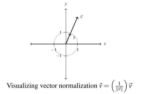
In part 3d of Example 9.1.4, we saw that the length of the direction vector, , . Vectors of length  play such an important role that they are given a special name.
Definition 9.5
Let be a vector. If  , then we say that is a unit vector.
Note that if is a unit vector, then necessarily,  . Conversely, in the solution of part 3d of Example 9.1.4, two different arguments show for any nonzero vector ,
  , so is a unit vector.
In other words, unit vectors are direction vectors and vice-versa. Indeed, the vector which we have defined as `the directional vector of ‘ is often described as `the unit vector in the direction of .’
In practice, if is a unit vector we write it as as opposed to because we have reserved the ` ‘ notation for unit vectors. The process of multiplying a nonzero vector by the factor to produce a unit vector is called `normalizing the vector.’
The terminal points of unit vectors, when plotted in standard position, lie on the Unit Circle. (You should take the time to show this.) As a result, we visualize normalizing a nonzero vector as shrinking[16] its terminal point, when plotted in standard position, back to the Unit Circle.
Of all of the unit vectors, two deserve special mention.

Geometrically, in the  -plane, the vector
  as represents the positive -direction, whereas the vector
  represents the positive -direction. We have the following `decomposition’ theorem.[17]
 .
.The proof of Theorem 9.4 is straightforward. Given  and
and  , we have from the definition of scalar multiplication and vector addition that
![\[ \begin{array}{rcl} v_{1} \bm\hat{\text{i}} + v_{2} \bm\hat{\text{j}} &=& v_{1}\left<1,0\right> + v_{2}\left<0,1\right>\\ &=& \left<v_{1},0\right> + \left<0,v_{2}\right> \\ &=& \left<v_{1},v_{2}\right> \\ &=& \vec{v} \end{array}\]](https://odp.library.tamu.edu/app/uploads/quicklatex/quicklatex.com-67401eef125d016473b031eb45c11491_l3.png "Rendered by QuickLaTeX.com")
Geometrically, the situation looks like this:
We conclude this section with a classic example which demonstrates how vectors are used in physics to study forces. A `force’ is defined as a `push’ or a `pull.’ The intensity of the push or pull is the magnitude of the force, and is measured in Newtons (N) in the SI system or pounds (lbs.) in the English system.[18]
The following example uses all of the concepts in this section, and should be studied in great detail.
Example 9.1.6
Example 9.1.6
A  pound speaker is suspended from the ceiling by two support braces. If one of them makes a angle with the ceiling and the other makes a
  angle with the ceiling, what are the tensions on each of the supports?
Solution:
We represent the problem schematically below along with the corresponding vector diagram.
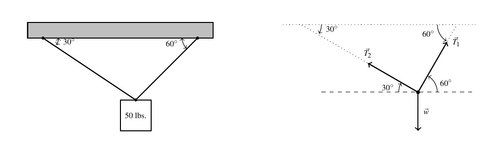
We have three forces acting on the speaker: the weight of the speaker, which we’ll call , pulling the speaker directly downward, and the forces on the support rods, which we’ll call  and
and  (for `tensions’) acting upward at angles and , respectively.
We are looking for the tensions on the support, which are the magnitudes  and
and  . In order for the speaker to remain stationary,[19] we require
  .
.
Viewing the common initial point of these vectors as the origin and the dashed line as the -axis, we use Theorem 9.3 to get component representations for the three vectors involved. We can model the weight of the speaker as a vector pointing directly downwards with a magnitude of 50 pounds. That is,  and
and  .
.
Hence,
![\[ \begin{array}{rcl} \vec{w} &=& 50\left<0,-1\right>\\ &=& \left<0,-50\right> \end{array} \]](https://odp.library.tamu.edu/app/uploads/quicklatex/quicklatex.com-486674e2b8c01bc3bbdbb9d57248eff9_l3.png "Rendered by QuickLaTeX.com")
For the force in the first support, we get
![\[ \begin{array}{rcl} \vec{T_{1}} & = & \| \vec{T_{1}} \|\left<\cos\left(60^{\circ}\right), \sin\left(60^{\circ}\right)\right> \\ [8pt] & = & \left< \dfrac{\| \vec{T_{1}} \|}{2} , \dfrac{\| \vec{T_{1}} \|\sqrt{3}}{2}\right> \\ \end{array} \]](https://odp.library.tamu.edu/app/uploads/quicklatex/quicklatex.com-77761dcb2452aecabc0d8bc4250d3dec_l3.png "Rendered by QuickLaTeX.com")
For the second support, we note that the angle is measured from the negative -axis, so the angle needed to write in component form is  . Hence
![\[ \begin{array}{rcl} \vec{T_{2}} & = & \| \vec{T_{2}} \|\left<\cos\left(150^{\circ}\right), \sin\left(150^{\circ}\right)\right>\\ [8pt] & = & \left<-\dfrac{\| \vec{T_{2}} \|\sqrt{3}}{2}, \dfrac{\| \vec{T_{2}} \|}{2} \right> \\ \end{array} \]](https://odp.library.tamu.edu/app/uploads/quicklatex/quicklatex.com-aea1ada71ee567aadce39f96d046c8c8_l3.png "Rendered by QuickLaTeX.com")
The requirement gives us the vector equation:
![\[ \begin{array}{rcl} \vec{w} + \vec{T_{1}} + \vec{T_{2}} & = & \vec{0} \\ [8pt] \left<0,-50\right> + \left< \dfrac{\| \vec{T_{1}} \|}{2} , \dfrac{\| \vec{T_{1}} \|\sqrt{3}}{2}\right> + \left<-\dfrac{\| \vec{T_{2}} \|\sqrt{3}}{2}, \dfrac{\| \vec{T_{2}} \|}{2} \right> & = & \left<0, 0\right> \\ [8pt] \left< \dfrac{\| \vec{T_{1}} \|}{2} -\dfrac{\| \vec{T_{2}} \|\sqrt{3}}{2}, \dfrac{\| \vec{T_{1}} \|\sqrt{3}}{2} + \dfrac{\| \vec{T_{2}} \|}{2} -50 \right> & = & \left<0, 0\right> \\ \end{array} \]](https://odp.library.tamu.edu/app/uploads/quicklatex/quicklatex.com-8378b7050316a01410f41475ae809eea_l3.png "Rendered by QuickLaTeX.com")
Equating the corresponding components of the vectors on each side, we get a system of linear equations in the variables and 
![\[\left\{ \begin{array}{lrcl} (E1) & \dfrac{\| \vec{T_{1}} \|}{2} -\dfrac{\| \vec{T_{2}} \|\sqrt{3}}{2} & = & 0 \\ [8pt] (E2) & \dfrac{\| \vec{T_{1}} \|\sqrt{3}}{2} + \dfrac{\| \vec{T_{2}} \|}{2} -50 & = & 0 \\ \end{array} \right.\]](https://odp.library.tamu.edu/app/uploads/quicklatex/quicklatex.com-5b6b818434a78779c9bc9421390f4636_l3.png "Rendered by QuickLaTeX.com")
From  , we get
  .
.
Substituting that into  gives
gives 
Solving, we get  , so
, so  pounds.
Hence,  pounds.
Note that the sum of the tensions on the wires in Example 9.1.6 exceed the pounds of the speaker. Explaining why this happens is a good exercise and gets at the heart of the concept of vectors and resolution of forces. Speaking of exercises 
9.1.1 Section Exercises
In Exercises 1 – 10, use the given pair of vectors and to compute the following quantities. State whether the result is a vector or a scalar.


Finally, verify that the vectors satisfy the Parallelogram Law
![\[ \|\vec{v}\|^2 + \|\vec{w}\|^2 = \dfrac{1}{2}\left[ \| \vec{v} + \vec{w}\|^2 + \|\vec{v} - \vec{w}\|^2\right] \]](https://odp.library.tamu.edu/app/uploads/quicklatex/quicklatex.com-58e05a41b0a11500c41aff15e0c84ca8_l3.png "Rendered by QuickLaTeX.com")
 ,
, 
 ,
, 
 ,
, 
 ,
, 
 ,
, 
 ,
, 
 ,
, 
 ,
, 
 ,
, 
 ,
, 
In Exercises 11 – 25, write the component form of the vector using the information given about its magnitude and direction. Give exact values.
 ; when drawn in standard position lies in Quadrant I and makes a angle with the positive -axis
 ; when drawn in standard position lies in Quadrant I and makes a
  angle with the positive -axis
 ; when drawn in standard position lies in Quadrant I and makes a angle with the positive -axis
 ; when drawn in standard position lies along the positive -axis
 ; when drawn in standard position lies in Quadrant II and makes a angle with the negative -axis
 ; when drawn in standard position lies in Quadrant II and makes a angle with the positive -axis
 ; when drawn in standard position lies along the negative -axis
 ; when drawn in standard position lies in Quadrant III and makes a angle with the negative -axis
 ; when drawn in standard position lies along the negative -axis
 ; when drawn in standard position lies in Quadrant IV and makes a angle with the positive -axis
 ; when drawn in standard position lies in Quadrant IV and makes a angle with the negative -axis
 ; when drawn in standard position lies in Quadrant I and makes an angle measuring
  with the positive -axis
 ; when drawn in standard position lies in Quadrant II and makes an angle measuring
  with the negative -axis
 ; when drawn in standard position lies in Quadrant III and makes an angle measuring
  with the negative -axis
 ; when drawn in standard position lies in Quadrant IV and makes an angle measuring
  with the positive -axis
In Exercises 26 – 31, approximate the component form of the vector using the information given about its magnitude and direction. Round your approximations to two decimal places.
 ; when drawn in standard position makes a
  angle with the positive -axis
 ; when drawn in standard position makes a
  angle with the positive -axis
 ; when drawn in standard position makes a
  angle with the positive -axis
 ; when drawn in standard position makes a
  angle with the positive -axis
 ; when drawn in standard position makes a
  angle with the positive -axis
- ; when drawn in standard position makes a
 angle with the positive -axis
In Exercises 32- 52, for the given vector , compute the magnitude and the direction angle with  so that
  (See Definition 9.4.) Round approximations to two decimal places.


- A small boat leaves the dock at Camp DuNuthin and heads across the Nessie River at 17 miles per hour (that is, with respect to the water) at a bearing of S
 W. The river is flowing due east at 8 miles per hour. What is the boat’s true speed and heading? Round the speed to the nearest mile per hour and express the heading as a bearing, rounded to the nearest tenth of a degree.
 - The HMS Sasquatch leaves port with bearing S
 E maintaining a speed of 42 miles per hour (that is, with respect to the water). If the ocean current is 5 miles per hour with a bearing of NE, find the HMS Sasquatch’s true speed and bearing. Round the speed to the nearest mile per hour and express the heading as a bearing, rounded to the nearest tenth of a degree.
 - If the captain of the HMS Sasquatch in Exercise 54 wishes to reach Chupacabra Cove, an island 100 miles away at a bearing of SE from port, in three hours, what speed and heading should she set to take into account the ocean current? Round the speed to the nearest mile per hour and express the heading as a bearing, rounded to the nearest tenth of a degree.
HINT: If denotes the velocity of the HMS Sasquatch and denotes the velocity of the current, what does need to be to reach Chupacabra Cove in three hours? - In calm air, a plane flying from the Pedimaxus International Airport can reach Cliffs of Insanity Point in two hours by following a bearing of N
 E at 96 miles an hour. (The distance between the airport and the cliffs is 192 miles.) If the wind is blowing from the southeast at 25 miles per hour, what speed and bearing should the pilot take so that she makes the trip in two hours along the original heading? Round the speed to the nearest hundredth of a mile per hour and your angle to the nearest tenth of a degree.
 - The SS Bigfoot leaves Yeti Bay on a course of N
 W at a speed of 50 miles per hour. After traveling half an hour, the captain determines he is 30 miles from the bay and his bearing back to the bay is SE. What is the speed and bearing of the ocean current? Round the speed to the nearest mile per hour and express the heading as a bearing, rounded to the nearest tenth of a degree.
 - A
 pound Sasquatch statue is suspended by two cables from a gymnasium ceiling. If each cable makes a angle with the ceiling, find the tension on each cable. Round your answer to the nearest pound.
 - Two cables are to support an object hanging from a ceiling. If the cables are each to make a
 angle with the ceiling, and each cable is rated to withstand a maximum tension of
  pounds, what is the heaviest object that can be supported? Round your answer down to the nearest pound.
 - A
 pound metal star is hanging on two cables which are attached to the ceiling. The left hand cable makes a
  angle with the ceiling while the right hand cable makes a
  angle with the ceiling. What is the tension on each of the cables? Round your answers to three decimal places.
 - Two drunken college students have filled an empty beer keg with rocks and tied ropes to it in order to drag it down the street in the middle of the night. The stronger of the two students pulls with a force of 100 pounds at a heading of N
 E and the other pulls at a heading of SE. What force should the weaker student apply to his rope so that the keg of rocks heads due east? What resultant force is applied to the keg? Round your answer to the nearest pound.
 - Emboldened by the success of their late night keg pull in Exercise 61 above, our intrepid young scholars have decided to pay homage to the chariot race scene from the movie `Ben-Hur’ by tying three ropes to a couch, loading the couch with all but one of their friends and pulling it due west down the street. The first rope points N
 W, the second points due west and the third points SW. The force applied to the first rope is 100 pounds, the force applied to the second rope is 40 pounds and the force applied (by the non-riding friend) to the third rope is 160 pounds. They need the resultant force to be at least 300 pounds otherwise the couch won’t move. Does it move? If so, is it heading due west?
 - Let
 be any non-zero vector. Show that
  has length 1.
 - We say that two non-zero vectors and are parallel if they have same or opposite directions. That is, and
 are parallel if either
  or
or  . Show that this means
  for some non-zero scalar and that if the vectors have the same direction and if they point in opposite directions.
 - The goal of this exercise is to use vectors to describe non-vertical lines in the plane. To that end, consider the line
 . Let
. Let  and let
  . Let
. Let  be any real number. Show that the vector defined by
  , when drawn in standard position, has its terminal point on the line . (Hint: Show that
  for any real number .) Now consider the non-vertical line
  . Repeat the previous analysis with
  and let
  . Thus any non-vertical line can be thought of as a collection of terminal points of the vector sum of
  (the position vector of the -intercept) and a scalar multiple of the slope vector .
 - Prove the associative and identity properties of vector addition in Theorem 9.1.
- Prove the properties of scalar multiplication in Theorem 9.2.
Section 9.1 Exercise Answers can be found in the Appendix … Coming soon
- The word `vector' comes from the Latin vehere meaning `to convey' or `to carry.' ↵
- Other textbook authors use bold vectors such as
 . We find that writing in bold font on the chalkboard is inconvenient at best, so we have chosen the `arrow' notation. ↵
 - If this idea of `over' and `up' seems familiar, it should. The slope of the line segment containing is
 . ↵
. ↵ - If necessary, review Sections 8.4.1 and 8.5. ↵
- That is, the speed of the plane relative to the air around it. If there were no wind, plane's airspeed would be the same as its speed as observed from the ground. How does wind affect this? Keep reading! ↵
- See Section 7.1.3, for instance. ↵
- Or, as our given angle, , is obtuse, we could use the Law of Sines without any ambiguity here. ↵
- In more advanced courses. chief among them Linear Algebra, vectors are actually defined as
 or
or  matrices, depending on the situation. ↵
 - Recall, is represented geometrically as a point ↵
- We will see in Definition 9.5 that we also call
 the unit vector in the direction of . ↵
 - Of course, to go from to
 , we are essentially `dividing both sides' of the equation by the scalar . The authors encourage the reader, however, to work out the details carefully to gain an appreciation of the properties in play. ↵
 - Due to the utility of vectors in `real-world' applications, we will usually use degree measure for the angle when giving the vector's direction. There are examples and exercises in which radians are used as well. ↵
- Keeping things `calculator' friendly, for once! ↵
- Yes, a calculator approximation is the quickest way to see this, but you can also use good old-fashioned inequalities and the fact that
 . ↵
. ↵ - We could just have easily used arcsine or arccosine here ↵
- if
 ↵
↵ - We will see a generalization of Theorem 9.4 in Section 9.2. Stay tuned! ↵
- See also Section 8.3.3. ↵
- This is the criteria for `static equilbrium'. ↵
The form of a vector, where the first component is the distance between x-coordinates and the second component is the distance between y-coordinates
A vector whose initial point is at (0,0).
A vector of length 1
