
5.1 Inverse Functions
In Section 1.2, we defined functions as processes. In this section, we seek to reverse, or `undo’ those processes. As in real life, we will find that some processes (like putting on socks and shoes) are reversible while some (like baking a cake) are not.
Consider the function  . Starting with a real number input
  , we apply two steps in the following sequence: first we multiply the input by
  and, second, we add
  to the result.
To reverse this process, we seek a function  which will undo each of these steps and take the output from
  ,
,  , and return the input . If we think of the two-step process of first putting on socks then putting on shoes, to reverse the process, we first take off the shoes and then we take off the socks. In much the same way, the function should undo each step of but in the opposite order. That is, the function should first subtract from the input then divide the result by . This leads us to the formula
  .
.
Let’s check to see if the function does the job. If  , then
  . Taking the output 19 from , we substitute it into to get
  , which is our original input to . To check that does the job for all in the domain of , we take the generic output from , , and substitute that into . That is, we simplify
  , which is our original input to . If we carefully examine the arithmetic as we simplify
  , we actually see first `undoing’ the addition of , and then `undoing’ the multiplication by .
Not only does undo , but also undoes . That is, if we take the output from , , and substitute that into , we get  . Using the language of function composition developed in Section 1.5.2, the statements
  and
and  can be written as
  and
and  , respectively.[1] Abstractly, we can visualize the relationship between and in the diagram below.
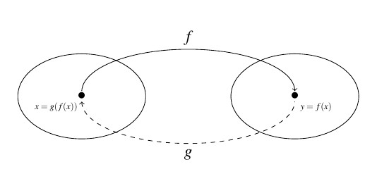
The main idea to get from the diagram is that takes the outputs from and returns them to their respective inputs, and conversely, takes outputs from and returns them to their respective inputs. We now have enough background to state the central definition of the section.
Definition 5.1
Suppose and are two functions such that
- for all in the domain of and
- for all in the domain of
then and are inverses of each other and the functions and are said to be invertible.
If we abstract one step further, we can express the sentiment in Definition 5.1 by saying that and are inverses if and only if  and
and  where
where  is the identity function restricted[2] to the domain of and
  is the identity function restricted to the domain of .
In other words,  for all in the domain of and
  for all in the domain of . Using this description of inverses along with the properties of function composition listed in Theorem 1.6, we can show that function inverses are unique.[3]
Suppose and  are both inverses of a function . By Theorem 5.1, the domain of is equal to the domain of , because both are the range of . This means the identity function applies both to the domain of and the domain of
  Thus
Thus
![\[ \begin{array}{rcl} h &=& h \circ I_{2} \\ &=& h \circ (f \circ g) \\ &=& (h \circ f) \circ g \\ &=& I_{1} \circ g \\ &=& g \end{array}\]](https://odp.library.tamu.edu/app/uploads/quicklatex/quicklatex.com-6f3634e709ed18fc621d5df453ace689_l3.png "Rendered by QuickLaTeX.com")
as required.
We summarize the important properties of invertible functions in the following theorem. Apart from introducing notation, each of the results below are immediate consequences of the idea that inverse functions map the outputs from a function back to their corresponding inputs.
Theorem 5.1 Properties of Inverse Functions
Suppose is an invertible function.
- There is exactly one inverse function for , denoted
 (read `-inverse’)
 - The range of is the domain of and the domain of is the range of
 if and only if
NOTE: In particular, for all in the range of , the solution to
  is
is 
 is on the graph of if and only if
  is on the graph of
NOTE: This means graph of is the reflection of the graph of
  across
  .[4]
.[4]- is an invertible function and

The notation is an unfortunate choice because you’ve been programmed since Algebra I to think of this as  . This is most definitely not the case, for instance, has as its inverse
  , which is certainly different than
Why does this confusing notation persist? As we mentioned in Section 1.5.2, the identity function  is to function composition what the real number
  is to real number multiplication. The choice of notation alludes to the property that
  and
and  , in much the same way as
  and
and  .
.
Before we embark on an example, we demonstrate the pertinent parts of Theorem 5.1 to the inverse pair and  . Suppose we wanted to solve
  . Going through the usual machinations, we obtain
  .
.
If we view this equation as  , however, then we are looking for the input corresponding to the output . This is exactly the question was built to answer. In other words, the solution to is
  . In other words, the formula
  encodes all of the algebra required to `undo’ what the formula
  does to . More generally, any time you have ever solved an equation, you have really been working through an inverse problem.
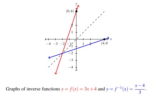
We also note the graphs of and are easily seen to be reflections across the line , as seen below. In particular, note that the -intercept  on the graph of
  corresponds to the -intercept on the graph of
  . Indeed, the point on the graph of can be interpreted as
  just as the point
  on the graph of can be interpreted as
  .
.
Example 5.1.1
Example 5.1.1.1
For each pair of functions and below:
![f(x) = \sqrt[3]{x-1} + 2](https://odp.library.tamu.edu/app/uploads/quicklatex/quicklatex.com-65f05cefea62582f8010fa7c250868fa_l3.png "Rendered by QuickLaTeX.com") and
and 
- Verify each pair of functions and are inverses: (a) algebraically and (b) graphically.
- Use the fact and are inverses to solve
 and
and 
Solution:
Solution for and .
-
- (a) To verify and are inverses, we appeal to Definition 5.1 and show and for all real numbers, .
![\[\begin{array}{lcl} \begin{array}{rcl} (g \circ f)(x) & = & g(f(x)) \\ & = & g(\sqrt[3]{x-1} + 2) \\ & = & [ (\sqrt[3]{x-1} + 2)-2]^3 + 1 \\ & = & (\sqrt[3]{x-1})^3 + 1 \\ & = & x-1+1 \\ & = & x \, \, \checkmark \\ \end{array} & \qquad & \begin{array}{rcl} (f \circ g)(x) & = & f(g(x)) \\ & = & f((x-2)^3+1) \\ & = & \sqrt[3]{[(x-2)^3+1] -1}+2 \\ & = & \sqrt[3]{(x-2)^3} +2\\ & = & x-4+4 \\ & = & x \, \, \checkmark \\ \end{array} \\ \end{array} \]](https://odp.library.tamu.edu/app/uploads/quicklatex/quicklatex.com-316c2600610482ec83d0a1fcfd981cf8_l3.png "Rendered by QuickLaTeX.com")
As the root here,
, is odd, Theorem 4.2 gives ![(\sqrt[3]{x-1})^3 = x-1](https://odp.library.tamu.edu/app/uploads/quicklatex/quicklatex.com-0d68fbf4e37c56a1af2ca0ebdd1bfe60_l3.png "Rendered by QuickLaTeX.com") and
and ![\sqrt[3]{(x-2)^3} = x-2](https://odp.library.tamu.edu/app/uploads/quicklatex/quicklatex.com-e5f9bf12cb72eb389522a64676daa3d9_l3.png "Rendered by QuickLaTeX.com") .
.
(b) To show and are inverses graphically, we graph and  on the same set of axes and check to see if they are reflections about the line .
The graph of![y = f(x) = \sqrt[3]{x-1} + 2](https://odp.library.tamu.edu/app/uploads/quicklatex/quicklatex.com-af5303b82e63871942f90c554a00e6d0_l3.png "Rendered by QuickLaTeX.com") appears below on the left courtesy of Theorem 4.1 in Section 4.1. The graph of
appears below on the left courtesy of Theorem 4.1 in Section 4.1. The graph of  appears below in the middle thanks to Theorem 2.2 in Section 2.2.
We can immediately see three pairs of corresponding points: and
and  ,
,  and
and  ,
,  and
and  . When graphed on the same pair of axes, the two graphs certainly appear to be symmetric about the line , as required.
- and are inverses, so the solution to is
 . To check, we find
 ![f(28) = \sqrt[3]{28-1}+2 = \sqrt[3]{27} + 2 = 3+2 = 5](https://odp.library.tamu.edu/app/uploads/quicklatex/quicklatex.com-8546a3ab884ee6a4964666ae9dd573da_l3.png "Rendered by QuickLaTeX.com") , as required.
, as required.
Likewise, the solution to is ![x = g^{-1}(-3) = f(-3) = \sqrt[3]{(-3)-1} + 2 = 2 - \sqrt[3]{4}](https://odp.library.tamu.edu/app/uploads/quicklatex/quicklatex.com-156643bbca0a956ddfebc1cf110f9a21_l3.png "Rendered by QuickLaTeX.com") . Once again, to check, we find
. Once again, to check, we find ![g(2 - \sqrt[3]{4}) = (2 - \sqrt[3]{4}-2)^3 + 1 = (-\sqrt[3]{4})^3 +1 = -4+1 = -3](https://odp.library.tamu.edu/app/uploads/quicklatex/quicklatex.com-6d523b408a8aec7a6ac378f0e5081ed3_l3.png "Rendered by QuickLaTeX.com") .
.
- (a) To verify
Example 5.1.1.2
For each pair of functions and below:
 and
and 
- Verify each pair of functions and are inverses: (a) algebraically and (b) graphically.
- Use the fact and are inverses to solve and
Solution:
Solution for and .
- (a) Note the domain of excludes
 and the domain of excludes
  . Hence, when simplifying
  and
and  , we tacitly assume
  and
and  , respectively.
![\[\begin{array}{ccc} \begin{array}{rcl} (g \circ f)(t) & = & g(f(t)) \\ [6pt] & = & g \left(\dfrac{2t}{t+1} \right) \\ [10pt] & = & \dfrac{\dfrac{2t}{t+1} }{2 - \dfrac{2t}{t+1}} \\ [25pt] & = & \dfrac{\dfrac{2t}{t+1} }{2 - \dfrac{2t}{t+1}} \cdot \dfrac{(t+1)}{(t+1)} \\ [25pt] & = & \dfrac{2t}{2(t+1) - 2t} \\ [10pt] & = & \dfrac{2t}{2t+2-2t} \\ [8pt] & = & \dfrac{2t}{2} \\ [8pt] & = & t \, \, \checkmark \\ \end{array} & \qquad & \begin{array}{rcl} (g \circ f)(t) & = & g(f(t)) \\ [6pt] & = & g \left(\dfrac{2t}{t+1} \right) \\ [10pt] & = & \dfrac{\dfrac{2t}{t+1} }{2 - \dfrac{2t}{t+1}} \\ [25pt] & = & \dfrac{\dfrac{2t}{t+1} }{2 - \dfrac{2t}{t+1}} \cdot \dfrac{(t+1)}{(t+1)} \\ [25pt] & = & \dfrac{2t}{2(t+1) - 2t} \\ [10pt] & = & \dfrac{2t}{2t+2-2t} \\ [8pt] & = & \dfrac{2t}{2} \\ [8pt] & = & t \, \, \checkmark \\ \end{array} \\ \end{array} \]](https://odp.library.tamu.edu/app/uploads/quicklatex/quicklatex.com-9fc2ccb071628dedeae9b988e8b4e97a_l3.png "Rendered by QuickLaTeX.com")
(b) We graph
 and
and  using the techniques discussed in Sections 3.2 and 3.3.
We find the graph of
has a vertical asymptote  and a horizontal asymptote
  . Corresponding to the vertical asymptote on the graph of , we find the graph of has a horizontal asymptote
Likewise, the horizontal asymptote
 on the graph of corresponds to the vertical asymptote on the graph of . Both graphs share the intercept
  . When graphed together on the same set of axes, the graphs of and do appear to be symmetric about the line
- Don’t let the fact that and in this case were defined using the independent variable, `
 ‘ instead of `‘ deter you in your efforts to solve . Remember that, ultimately, the function here is the process represented by the formula
  , and is the same process (with the same inverse!) regardless of the letter used as the independent variable. Hence, the solution to is
  . We get
  .
.
To check, we find . Similarly, we solve by finding
  . Sure enough, we find
  .
.
We now investigate under what circumstances a function is invertible. As a way to motivate the discussion, we consider  . A likely candidate for the inverse is the function
  . However,
  , which is not equal to unless
  . For example, when
  ,
,  , but
, but  . That is, failed to return the input
  from its output . Instead, matches the output to a different input, namely
  , which satisfies
  . Schematically:
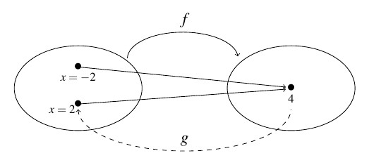
We see from the diagram that both  and
and  are , thus it is impossible to construct a function which takes back to both
  and . Recall that by definition, a function can match with only one number.
In general, in order for a function to be invertible, each output can come from only one input. By definition, a function matches up each input to only one output, thus invertible functions have the property that they match one input to one output and vice-versa. We formalize this concept below.
Definition 5.2
A function is said to be one-to-one if whenever  , then
Note that an equivalent way to state Definition 5.2 is that a function is one-to-one if different inputs go to different outputs. That is, if  , then
Before we solidify the connection between invertible functions and one-to-one functions, we take a moment to see what goes wrong graphically when trying to find the inverse of .
Per Theorem 5.1, the graph of , if it exists, is obtained from the graph of  by reflecting about the line . Procedurally, this is accomplished by interchanging the and coordinates of each point on the graph of
  . Algebraically, we are swapping the variables `‘ and `‘ which results in the equation
  whose graph is below on the right.

We see immediately the graph of fails the Vertical Line Test, Theorem 1.2. In particular, the vertical line  intersects the graph at two points,
  and
and  meaning the relation described by matches the -value with two different -values, and .
Note that the vertical line and the points  on the graph of
  correspond to the horizontal line
  and the points
  on the graph of which brings us right back to the concept of one-to-one. The fact that both
  and
and  are on the graph of means
  . Hence, takes different inputs, and , to the same output, , so is not one-to-one.
Recall the Horizontal Line Test from Exercise57 in Section 1.2. Applying that result to the graph of we say the graph of `fails’ the Horizontal Line Test because the horizontal line intersects the graph of more than once. This means that the equation does not represent as a function of .
Said differently, the Horizontal Line Test detects when there is at least one -value () which is matched to more than one -value ( ). In other words, the Horizontal Line Test can be used to detect whether or not a function is one-to-one.
So, to review, is not invertible, not one-to-one, and its graph fails the Horizontal Line Test. It turns out that these three attributes: being invertible, one-to-one, and having a graph that passes the Horizontal Line Test are mathematically equivalent. That is to say if one if these things is true about a function, then they all are; it also means that, as in this case, if one of these things isn’t true about a function, then none of them are. We summarize this result in the following theorem.
Theorem 5.2 Equivalent Conditions for Invertibility
For a function , either all of the following statements are true or none of them are:
- is invertible.
- The graph of passes the Horizontal Line Test.[5]
To prove Theorem 5.2, we first suppose is invertible. Then there is a function so that for all in the domain of . If , then  . As a result of , the equation reduces to
  . We’ve shown that if , then , proving is one-to-one.
Next, assume is one-to-one. Suppose a horizontal line  intersects the graph of at the points and
  . This means and
  so . Because is one-to-one, means
  so the points and are actually one in the same. This establishes that each horizontal line can intersect the graph of at most once, so the graph of passes the Horizontal Line Test.
Last, but not least, suppose the graph of passes the Horizontal Line Test. Let  be a real number in the range of . Then the horizontal line intersects the graph of just once, say at the point
  . Define the mapping so that
  . The mapping is a function because each horizontal line where is in the range of intersects the graph of only once. By construction, we have the domain of is the range of and that for all in the domain of , . We leave it to the reader to show that for all in the domain of , , too.
Hence, we’ve shown: first, if invertible, then is one-to-one; second, if is one-to-one, then the graph of passes the Horizontal Line Test; and third, if passes the Horizontal Line Test, then is invertible. Therefore if is satisfies any one of these three conditions, then must satisfy the other two.[6]
We put this result to work in the next example.
Example 5.1.2
Example 5.1.2.1
Determine if the following functions are one-to-one:
- analytically using Definition 5.2 and
- graphically using the Horizontal Line Test.
For the functions that are one-to-one, graph the inverse.

Solution:
Determine if is a one-to-one function.
- To determine whether or not is one-to-one analytically, we assume and work to see if we can deduce . As we work our way through the problem, we encounter a quadratic equation. We rewrite the equation so it equals
 and factor by grouping. We get as one possibility, but we also get the possibility that
  . This suggests that may not be one-to-one. Taking
  , we get
  or
or  . We have two different inputs with the same output as
  and , proving is neither one-to-one nor invertible.
![\[ \begin{array}{rcl} f(a) & = & f(b) \\ a^2 - 2a+4 & = & b^2 - 2b+4 \\ a^2 - 2a & = & b^2 - 2b \\ a^2 - b^2 - 2a + 2b & = & 0 \\ (a+b)(a-b) - 2(a-b) & = & 0 \\ (a-b)((a+b) -2) & = & 0 \\ a-b = 0 & \text{or} & a+b -2 = 0 \\ a = b & \text{or} & a = 2-b \\ \end{array} \]](https://odp.library.tamu.edu/app/uploads/quicklatex/quicklatex.com-5a93f67ca9b54ac071341e07ef467ad3_l3.png "Rendered by QuickLaTeX.com")
- We note that is a quadratic function and we graph using the techniques presented in Section 2.1. We see the graph fails the Horizontal Line Test quite often – in particular, crossing the line at the points and .

Example 5.1.2.2
Determine if the following functions are one-to-one:
- analytically using Definition 5.2 and
- graphically using the Horizontal Line Test.
For the functions that are one-to-one, graph the inverse.

Solution:
Determine if is a one-to-one function.
- We begin with the assumption that
 for
for  ,
,  in the domain of (That is, we assume
  and
and  .) Through our work, we deduce , proving is one-to-one.
![\[ \begin{array}{rcl} g(a) & = & g(b) \\ [3pt] \dfrac{2a}{1-a} & = & \dfrac{2b}{1-b} \\ [6pt] 2a(1-b) & = & 2b(1-a) \\ 2a - 2ab & = & 2b - 2ba \\ 2a & = & 2b \\ a & = & b \, \, \checkmark \\ \end{array} \]](https://odp.library.tamu.edu/app/uploads/quicklatex/quicklatex.com-073b399f2e885be83949c17759fbddc7_l3.png "Rendered by QuickLaTeX.com")
- We graph using the procedure outlined in Section 3.3. We find the sole intercept is with asymptotes
 and
and  . Based on our graph, the graph of appears to pass the Horizontal Line Test, verifying is one-to-one.

Because
is one-to-one, is invertible. Even though we do not have a formula for  , we can nevertheless sketch the graph of
  by reflecting the graph of across
  .
.Corresponding to the vertical asymptote
on the graph of , the graph of will have a horizontal asymptote  . Similarly, the horizontal asymptote
  on the graph of corresponds to a vertical asymptote
  on the graph of
  . The point remains unchanged when we switch the and coordinates, so it is on both the graph of and .
Example 5.1.2.3
Determine if the following functions are one-to-one:
- analytically using Definition 5.2 and
- graphically using the Horizontal Line Test.
For the functions that are one-to-one, graph the inverse.

Solution:
Determine if is a one-to-one function.
- The function
 is given to us as a set of ordered pairs. Recall each ordered pair is of the form
  . As
. As  and are both elements of , this means
  and
and  .
.
Hence, we have two distinct inputs, and with the same output, , thus is not one-to-one and, hence, not invertible.
 - To graph , we plot the points in below on the left. We see the horizontal line
 crosses the graph more than once. Hence, the graph of fails the Horizontal Line Test.

Example 5.1.2.4
Determine if the following functions are one-to-one:
- analytically using Definition 5.2 and
- graphically using the Horizontal Line Test.
For the functions that are one-to-one, graph the inverse.

Solution:
Determine if  is a one-to-one function.
Like the function above, the function  is described as a set of ordered pairs. Before we set about determining whether or not is one-to-one, we take a moment to show is, in fact, a function. That is, we must show that each real number input to is matched to only one output.
We are given . and we know that when represented in this way, each ordered pair is of the form (input, output). Hence, the inputs to are of the form  and the outputs from are of the form
  . To establish is a function, we must show that each input produces only one output. If it should happen that
  , then we must show
  . The equation gives
  , or . From this it follows that
  so is a function.
- To show is one-to-one, we must show that if two outputs from are the same, the corresponding inputs must also be the same. That is, we must show that if , then . We see almost immediately that if then so as required. This shows is one-to-one and, hence, invertible.
- We graph below on the left by plotting points in the default
 -plane by choosing different values for . For instance,
  corresponds to the point
  , corresponds to the point
  , corresponds to the point
  , etc. Our graph appears to pass the Horizontal Line Test, confirming is one-to-one. We obtain the graph of
  below on the right by reflecting the graph of about the line

In Example 5.1.2, we showed the functions and are invertible and graphed their inverses. While graphs are perfectly fine representations of functions, we have seen where they aren’t the most accurate. Ideally, we would like to represent and in the same manner in which and are presented to us. The key to doing this is to recall that inverse functions take outputs back to their associated inputs.
Consider  . As mentioned in Example 5.1.2, the ordered pairs which comprise are in the form (input, output). Hence to find a compatible description for , we simply interchange the expressions in each of the coordinates to obtain
  .
.
The function was defined in terms of a formula, so we would like to find a formula representation for . We apply the same logic as above. Here, the input, represented by the independent variable , and the output, represented by the dependent variable , are related by the equation  . Hence, to exchange inputs and outputs, we interchange the `‘ and `‘ variables. Doing so, we obtain the equation
  which is an implicit description for . Solving for gives an explicit formula for , namely . We demonstrate this technique below.
![\[ \begin{array}{rclr} y & = & g(t) & \\ [5pt] y & = & \dfrac{2t}{1-t} & \\ [7pt] t & = & \dfrac{2y}{1-y} & \text{interchange variables: } t \text{ and } y \\ [3pt] t(1-y) & = & 2y & \\ [3pt] t-ty & = & 2y & \\ [3pt] t & = & ty + 2y & \\ [3pt] t & = & y(t+2) & \text{factor}\\ [8pt] y & = & \dfrac{t}{t+2} \end{array} \]](https://odp.library.tamu.edu/app/uploads/quicklatex/quicklatex.com-254103ba34f9bc364e129d9b30983ccc_l3.png "Rendered by QuickLaTeX.com")
We claim  , and leave the algebraic verification of this to the reader.
We generalize this approach below. As always, we resort to the default `‘ and `‘ labels for the independent and dependent variables, respectively.
Steps for finding a formula for the inverse of a one-to-one function
- Write
- Interchange and
- Solve
 for to obtain
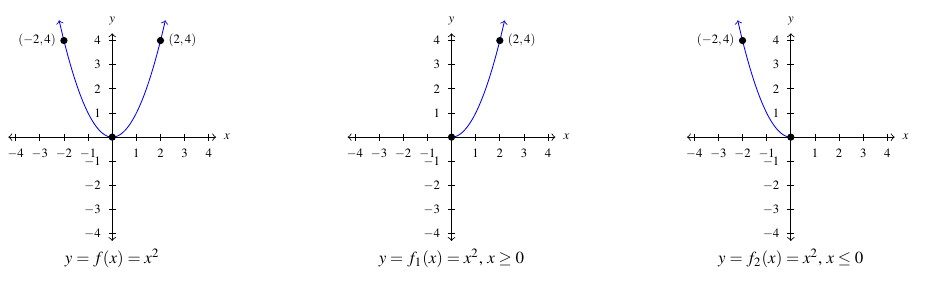
We now return to . We know that is not one-to-one, and thus, is not invertible, but our goal here is to see what goes wrong algebraically.
If we attempt to follow the algorithm above to find a formula for , we start with the equation and interchange the variables `‘ and `‘ to produce the equation . Solving for gives  It’s this `
 ‘ which is causing the problem for us as this produces two -values for any
Using the language of Section 1.2, the equation implicitly defines two functions,  and
and  , each of which represents the top and bottom halves, respectively, of the graph of
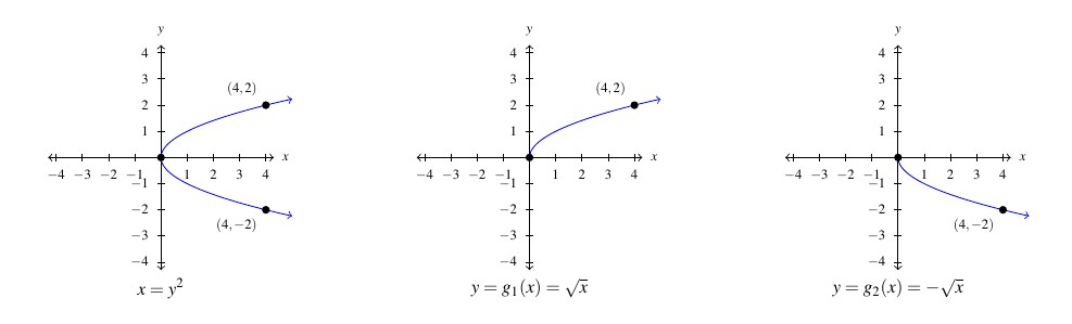
Hence, in some sense, we have two partial inverses for : returns the positive inputs from and returns the negative inputs to . In order to view each of these functions as strict inverses, however, we need to split into two parts:  for and
  for
for  .
.
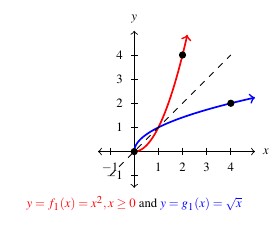
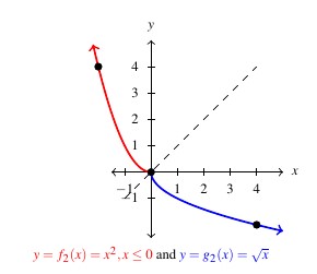
We claim that  and
and  are an inverse function pair as are
  and
and  . Indeed, we find:
![\[ \begin{array}{rcl} \begin{array}{rcl} (g_{1} \circ f_{1})(x) & = & g_{1}(f_{1}(x)) \\ & = & g_{1}(x^2) \\ & = & \sqrt{x^2} \\ & = & |x| = x, \, \text{as $x \geq 0$.} \\ \end{array} & \qquad \qquad & \begin{array}{rcl} (f_{1} \circ g_{1})(x) & = & f_{1}(g_{1}(x)) \\ & = & f_{1}(\sqrt{x}) \\ & = & (\sqrt{x})^2 \\ & = & x \\ \end{array} \\ \end{array} \]](https://odp.library.tamu.edu/app/uploads/quicklatex/quicklatex.com-d86762f8d4a62b7eca6a9ceb69bdf157_l3.png "Rendered by QuickLaTeX.com")
![\[ \begin{array}{rcl} \begin{array}{rcl} (g_{2} \circ f_{2})(x) & = & g_{2}(f_{2}(x)) \\ & = & g_{2}(x^2) \\ & = & -\sqrt{x^2} \\ & = & - |x| \\ & = & -(-x) = x, \, \text{as $x \leq 0$.} \end{array} & \qquad \qquad & \begin{array}{rcl} (f_{2} \circ g_{2})(x) & = & f_{2}(g_{2}(x)) \\ & = & f_{2}(-\sqrt{x}) \\ & = & (-\sqrt{x})^2 \\ & = & (\sqrt{x})^2 \\ & = & x \\ \end{array} \\ \end{array} \]](https://odp.library.tamu.edu/app/uploads/quicklatex/quicklatex.com-370b3168e7b1265d60ac4ea53e746856_l3.png "Rendered by QuickLaTeX.com")
Hence, by restricting the domain of we are able to produce invertible functions. Said differently, because the equation implicitly describes a pair of functions, the equation implicitly describes a pair of invertible functions.
Our next example continues the theme of restricting the domain of a function to find inverse functions.
Example 5.1.3
Example 5.1.3.1
Graph the following functions to show they are one-to-one and determine their inverses. Check your answers analytically using function composition and graphically.
 ,
, 
Solution:
Graph , to show it is one-to-one and determine its inverse.
The function  is a restriction of the function from Example 5.1.2. The domain of is restricted to , therefore we are selecting only the `left half’ of the parabola. Hence, the graph of , seen below, passes the Horizontal Line Test and thus is invertible.

Next, we find an explicit formula for  using our standard algorithm.[7]
![\[ \begin{array}{rclr} y & = & j(x) & \\ y & = & x^2-2x+4, \, \, \, x \leq 1 \\ x & = & y^2 - 2y+4, \, \, \, y \leq 1 & \text{switch } x \text{ and } y \\ 0 & = & y^2 - 2y + 4-x & \\ y & = & \dfrac{2 \pm \sqrt{(-2)^2-4(1)(4-x)}}{2(1)} & \text{quadratic formula, } c=4-x \\ [10pt] y & = & \dfrac{2 \pm \sqrt{4x-12}}{2} & \\ [6pt] y & = & \dfrac{2 \pm \sqrt{4(x-3)}}{2} & \\ [6pt] y & = & \dfrac{2 \pm 2\sqrt{x-3}}{2} & \\ [6pt] y & = & \dfrac{2\left(1 \pm \sqrt{x-3}\right)}{2} & \\ [6pt] y & = & 1 \pm \sqrt{x-3} & \\ y & = & 1 - \sqrt{x-3} & \text{due to the fact that } y \leq 1 \\ \end{array} \]](https://odp.library.tamu.edu/app/uploads/quicklatex/quicklatex.com-6e663ba1de2d9396d794126308441147_l3.png "Rendered by QuickLaTeX.com")
Hence,  .
.
To check our answer algebraically, we simplify  and
and  Note the importance of the domain restriction when simplifying .
![\[ \begin{array}{rcl} \left(j^{-1} \circ j \right)(x) & = & j^{-1}(j(x)) \\ & = & j^{-1}\left(x^2-2x+4\right), \, \, \, x \leq 1 \\ & = & 1 - \sqrt{\left(x^2-2x+4\right)-3} \\ & = & 1 - \sqrt{x^2-2x+1} \\ & = & 1 - \sqrt{(x-1)^2} \\ & = & 1 - |x-1| \\ & = & 1 - (-(x-1)) \, \, \text{as $x \leq 1$}\\ & = & x \, \, \checkmark \\ \end{array} \]](https://odp.library.tamu.edu/app/uploads/quicklatex/quicklatex.com-1764791f8bde16c7c70a825a9d2d2531_l3.png "Rendered by QuickLaTeX.com")
![\[ \begin{array}{rcl} \left(j \circ j^{-1} \right)(x) & = & j\left(j^{-1}(x)\right) \\ & = & j\left(1 - \sqrt{x-3}\right) \\ & = & \left(1 - \sqrt{x-3}\right)^2-2\left(1 - \sqrt{x-3}\right)+4 \\ & = & 1 - 2\sqrt{x-3} + \left(\sqrt{x-3}\right)^2 -2 \\ & & + \, 2\sqrt{x-3}+4 \\ & = & 1+ x-3 -2 +4 \\ & = & x \, \, \checkmark \\ \end{array} \]](https://odp.library.tamu.edu/app/uploads/quicklatex/quicklatex.com-f9fdc20e40c296d83d49351d07ea0140_l3.png "Rendered by QuickLaTeX.com")
We graph both and  on the axes below. They appear to be symmetric about the line .

Example 5.1.3.2
Graph the following functions to show they are one-to-one 2nd determine their inverses. Check your answers analytically using function composition and graphically.

Solution:
Graph to show it is one-to-one and determine its inverse.
Graphing  , we see
  is one-to-one,

so we proceed to find an formula for  .
.
![\[ \begin{array}{rclr} y & = & k(t) & \\ y & = & \sqrt{t+2}-1 & \\ t & = & \sqrt{y+2} - 1 & \text{switch $t$ and $y$} \\ t+1 & = & \sqrt{y+2} & \\ (t+1)^2 & = & \left(\sqrt{y+2}\right)^2 & \\ t^2 + 2t + 1 & = & y + 2 & \\ y & = & t^2 + 2t - 1 & \\ \end{array} \]](https://odp.library.tamu.edu/app/uploads/quicklatex/quicklatex.com-84e7ce1207d89a744ae6fd6a1ea79dc1_l3.png "Rendered by QuickLaTeX.com")
We have  . Based on our experience, we know something isn’t quite right. We determined is a quadratic function, and we have seen several times in this section that these are not one-to-one unless their domains are suitably restricted.
Theorem 5.1tells us that the domain of is the range of . From the graph of , we see that the range is  , which means we restrict the domain of to
  .
.
We now check that this works in our compositions. Note the importance of the domain restriction, when simplifying  .
.
![\[ \begin{array}{rcl} \left(k^{-1} \circ k \right)(t) & = & k^{-1}(k(t)) \\ & = & k^{-1}\left(\sqrt{t+2}-1\right) \\ & = & \left(\sqrt{t+2}-1\right)^2 + 2\left(\sqrt{t+2}-1\right) - 1 \\ & = & \left(\sqrt{t+2}\right)^2 - 2\sqrt{t+2} + 1 \\ && + \, 2 \sqrt{t+2} - 2 - 1 \\ & = &t+2 -2 \\ & = & t \, \, \checkmark \\ \end{array}\]](https://odp.library.tamu.edu/app/uploads/quicklatex/quicklatex.com-99a467102e938d9a9c151674ebeb5011_l3.png "Rendered by QuickLaTeX.com")
![\[\begin{array}{rcl} \left(k \circ k^{-1} \right)(t) & = & k\left( t^2+2t-1 \right), \, \, \, t \geq -1 \\ & = & \sqrt{\left(t^2+2t-1\right)+2}-1 \\ & = & \sqrt{t^2+2t+1}-1 \\ & = & \sqrt{(t+1)^2}-1 \\ & = & |t+1| -1 \\ & = & t+1 -1, \, \, \text{as $t \geq -1$} \\ & = & t \, \, \checkmark \\ \end{array} \]](https://odp.library.tamu.edu/app/uploads/quicklatex/quicklatex.com-1a61689367baa9dfcf0020faf6db959f_l3.png "Rendered by QuickLaTeX.com")
Graphically, everything checks out, provided that we remember the domain restriction on means we take the right half of the parabola.

Our last example of the section gives an application of inverse functions. Recall in Example 1.3.9 in Section 1.3.1, we modeled the demand for PortaBoy game systems as the price per system,  as a function of the number of systems sold, . In the following example, we find
  and interpret what it means.
Example 5.1.4
Example 5.1.4.1
Recall the price-demand function for PortaBoy game systems is modeled by the formula  for
for  where represents the number of systems sold (the demand) and is the price per system, in dollars.
Explain why  is one-to-one and find a formula for . State the restricted domain.
Solution:
Explain why is one-to-one and find a formula for . State the restricted domain.
Recall the graph of , , is a line segment from  to
to  , and as such passes the Horizontal Line Test. Hence, is one-to-one.
We determine the expression for as usual and get 
The domain of  should match the range of , which is
 ![[1,250]](https://odp.library.tamu.edu/app/uploads/quicklatex/quicklatex.com-cc4b02713a1711e3a22f1b86217d4c0d_l3.png "Rendered by QuickLaTeX.com") , and as such, we restrict the domain of to
, and as such, we restrict the domain of to 
Example 5.1.4.2
Recall the price-demand function for PortaBoy game systems is modeled by the formula for where represents the number of systems sold (the demand) and is the price per system, in dollars.
Compute and interpret  .
.
Solution:
Compute and interpret .
We find  .
.
The function took as inputs the number of systems sold and returned the price per system as the output, thus takes the price per system as its input and returns the number of systems sold as its output.
Hence,  means 20 systems will be sold if the price is set at 220 dollars per system.
Example 5.1.4.3
Recall the price-demand function for PortaBoy game systems is modeled by the formula for where represents the number of systems sold (the demand) and is the price per system, in dollars.
Recall from Section 2.1that the profit  , in dollars, as a result of selling systems is given by
  . Write and interpret
  .
.
Solution:
Write and interpret .
We compute
![\[ \begin{array}{rcl} \left( P \circ p^{-1}\right)(x) & = & P \left(p^{-1}(x)\right) \\ & = & P\left(\frac{500-2x}{3}\right) \\ & = & -1.5\left(\frac{500-2x}{3}\right)^2+170\left(\frac{500-2x}{3}\right)-150 \end{array} \]](https://odp.library.tamu.edu/app/uploads/quicklatex/quicklatex.com-ccfd9329030bb77df851c905f8dbef9d_l3.png "Rendered by QuickLaTeX.com")
After a hefty amount of algebra,[8] we obtain  .
.
To understand what this means, recall that the original profit function gave us the profit as a function of the number of systems sold. The function gives us the number of systems sold as a function of the price.
Hence, when we compute  , we input a price per system, into the function .
The number is the number of systems sold at that price. This number is then fed into to return the profit obtained by selling systems.
Hence,  gives us the profit (in dollars) as a function of the price per system, .
Example 5.1.4.4
Recall the price-demand function for PortaBoy game systems is modeled by the formula for where represents the number of systems sold (the demand) and is the price per system, in dollars.
Use your answer to part 3 to determine the price per PortaBoy which would yield the maximum profit. Compare with Example 2.1.3.
Solution:
Use your answer to part 3 to determine the price per PortaBoy which would yield the maximum profit. Compare with Example 2.1.3.
We know from Section 2.1 that the graph of  is a parabola opening downwards. The maximum profit is realized at the vertex. We are concerned only with the price per system, so we need only find the -coordinate of the vertex.
Identifying  and
and  , we get, by the Vertex Formula, Equation 2.1,
  .
.
Hence, the weekly profit is maximized if we set the price at 165 dollars per system. Comparing this with our answer from Example 2.1.3, there is a slight discrepancy to the tune of 50 cents. We leave it to the reader to balance the books appropriately.
5.1.1 Section Exercises
In Exercises 1 – 8, verify the given pairs of functions are inverses algebraically and graphically.
 and
and 
 and
and 
 and
and 
 and
and 
 and
and  ,
,  and
and  ,
,  and
and ![g(t) = \sqrt[3]{t-5}+1](https://odp.library.tamu.edu/app/uploads/quicklatex/quicklatex.com-f6f3e1d67a6aca8212e7e6fbfa418499_l3.png "Rendered by QuickLaTeX.com")
![f(t) = -\sqrt[4]{t-2}](https://odp.library.tamu.edu/app/uploads/quicklatex/quicklatex.com-1137a54249271c1e5be25942b930c049_l3.png "Rendered by QuickLaTeX.com") and
and  ,
, 
In Exercises 9 – 28, show that the given function is one-to-one and find its inverse. Check your answers algebraically and graphically. Verify the range of the function is the domain of its inverse and vice-versa.


![f(x) = \sqrt[5]{3x-1}](https://odp.library.tamu.edu/app/uploads/quicklatex/quicklatex.com-c0212e8c410768742802d1203f707166_l3.png "Rendered by QuickLaTeX.com")
![f(x) = 3-\sqrt[3]{x-2}](https://odp.library.tamu.edu/app/uploads/quicklatex/quicklatex.com-f06b094672d281ba4818510956f1e474_l3.png "Rendered by QuickLaTeX.com")
 ,
, 


 ,
, 


- Explain why each set of ordered pairs below represents a one-to-one function and find the inverse.

 NOTE: The difference between and is the `
 .’
.’
 [9]
[9]
In Exercises 30 – 33, explain why each graph represents[10] a one-to-one function and graph its inverse.
-

-


- The price of a dOpi media player, in dollars per dOpi, is given as a function of the weekly sales according to the formula
 for
for  .
.
- Find and state its domain.
- Compute and interpret
 .
. - The profit (in dollars) made from producing and selling dOpis per week is given by the formula
 , for . Find and determine what price per dOpi would yield the maximum profit. What is the maximum profit? How many dOpis need to be produced and sold to achieve the maximum profit?
- Find
- Show that the Fahrenheit to Celsius conversion function found in Exercise 67 in Section1.3.3 is invertible and that its inverse is the Celsius to Fahrenheit conversion function.
- Analytically show that the function
 is one-to-one. Use Theorem 5.1 to help you compute
  and
and  . What happens when you attempt to find a formula for ?
 - Let
 .
.
- Graph using the techniques in Section 3.3. Check your answer using a graphing utility.
- Verify that is one-to-one on the interval .
- Use the procedure outlined in this section to find the formula for for
 .
. - Because
 , it should be the case that
  . What goes wrong when you attempt to substitute
  into ? Discuss with your classmates how this problem arose and possible remedies.
- Graph
- The function given in number 4 is an example of a function which is its own inverse.
- Algebraically verify every function of the form:
 is its own inverse.What assumptions do you need to make about the values of , , and ?
 - Under what conditions is
 ,
,  its own inverse? Prove your answer.
- Algebraically verify every function of the form:
Section 5.1 Exercise Answers can be found in the Appendix … Coming soon
- At the level of functions,
 , where is the identity function as defined as
  for all real numbers, . ↵
 - The identity function , first introduced in Exercise 76 in Section 1.3.1 and mentioned in Theorem 1.6, has a domain of all real numbers. As the domains of and may not be all real numbers, we need the restrictions listed here. ↵
- In other words, invertible functions have exactly one inverse. ↵
- See Example 1.1.5 in Section 1.1 and Example 1.35 in Section 1.3.1. ↵
- i.e., no horizontal line intersects the graph more than once. ↵
- For example, if we know is one-to-one, we showed the graph of passes the HLT which, in turn, guarantees is invertible. ↵
- Here, we use the Quadratic Formula to solve for . For `completeness,' we note you can (and should!) also consider solving for by `completing' the square. ↵
- It is good review to actually do this! ↵
- Recall this means
 ↵
↵ - or, more precisely, appears to represent ↵
Two functions are inverses if their compositions are both true for all x.
A function is invertible if the function has an inverse.
A function is one-to-one if whenever f(a)=f(b), then a=b.
