8.2  Other Trigonometric Identities

Vanessa Coffelt

8.2 Other Trigonometric Identities

In Section 8.1, we saw the utility of identities in finding the values of the circular functions of a given angle as well as simplifying expressions involving the circular functions. In this section, we introduce several collections of identities which have uses in this course and beyond.

Our first set of identities is the `Even/Odd’ identities. We observed the even and odd properties of the circular functions graphically in Sections 7.3 and 7.5. Here, we take the time to prove these properties from first principles. We state the theorem below for reference.

Theorem 8.4 Even/Odd Identities

For all applicable angles $\theta$ ,

$\cos(-\theta) = \cos(\theta)$
$\sec(-\theta) = \sec(\theta)$
$\sin(-\theta) = -\sin(\theta)$
$\csc(-\theta) = -\csc(\theta)$
$\tan(-\theta) = -\tan(\theta)$
$\cot(-\theta) = -\cot(\theta)$

We start by proving $\cos(-\theta) = \cos(\theta)$ and $\sin(-\theta) = -\sin(\theta)$ .

Consider an angle $\theta$ plotted in standard position. Let $\theta_{0}$ be the angle coterminal with $\theta$ with $0 \leq \theta_{0} < 2\pi$ . (We can construct the angle $\theta_{0}$ by rotating counter-clockwise from the positive $x$ -axis to the terminal side of $\theta$ as pictured below.) $\theta$ and $\theta_{0}$ are coterminal, so $\cos(\theta) = \cos(\theta_{0})$ and $\sin(\theta) = \sin(\theta_{0}).$

Two unit circles side by side. The first unit circle has theta sub zero with a terminal side in the second quadrant. The angle is indicated with thicker lines. As a thinner line, theta is noted sharing the same terminal side, but rotating in a clockwise direction. The second unit circle has the same theta sub zero and also negative theta sub zero. The terminal sides are reflections across the x-axis. The point on the terminal side theta sub zero is P and the point on the terminal side of negative theta sub zero is Q. — Geometric Proof of Even and Odd Identities

We now consider the angles $-\theta$ and $-\theta_{0}$ . As $\theta$ is coterminal with $\theta_{\0}$ , there is some integer $k$ such that $\theta = \theta_{0} + 2\pi \cdot k$ . Hence, $-\theta = -\theta_{0} - 2\pi \cdot k = -\theta_{0} + 2\pi \cdot(-k)$ . Because $k$ is an integer, so is $(-k)$ , which means $-\theta$ is coterminal with $-\theta_{0}$ . Therefore, $\cos(-\theta) = \cos(-\theta_{0})$ and $\sin(-\theta) = \sin(-\theta_{0}).$

Let $P$ and $Q$ denote the points on the terminal sides of $\theta_{0}$ and $-\theta_{0}}$ , respectively, which lie on the Unit Circle. By definition, the coordinates of $P$ are $(\cos(\theta_{0}),\sin(\theta_{0}))$ and the coordinates of $Q$ are $(\cos(-\theta_{0}),\sin(-\theta_{0})).$

Because $\theta_{0}$ and $-\theta_{0}$ sweep out congruent central sectors of the Unit Circle, it follows that the points $P$ and $Q$ are symmetric about the $x$ -axis. Thus, $\cos(-\theta_{0}) = \cos(\theta_{0})$ and $\sin(-\theta_{0}) = -\sin(\theta_{0}).$

The cosines and sines of $\theta_{0}$ and $-\theta_{0}$ are the same as those for $\theta$ and $-\theta$ , respectively, thus we get $\cos(-\theta) = \cos(\theta)$ and $\sin(-\theta) = -\sin(\theta)$ , as required.

As we saw in Section 7.5, the remaining four circular functions `inherit’ their even/odd nature from sine and cosine courtesy of the Reciprocal and Quotient Identities, Theorem 8.1.

Our next set of identities establish how the cosine function handles sums and differences of angles.

Theorem 8.5 Sum and Difference Identities for Cosine

For all angles $\alpha$ and $\beta$ ,

$\cos(\alpha + \beta) = \cos(\alpha) \cos(\beta) - \sin(\alpha) \sin(\beta)$
$\cos(\alpha - \beta) = \cos(\alpha) \cos(\beta) + \sin(\alpha) \sin(\beta)$

We first prove the result for differences. As in the proof of the Even / Odd Identities, we can reduce the proof for general angles $\alpha$ and $\beta$ to angles $\alpha_{0}$ and $\beta_{0}$ , coterminal with $\alpha$ and $\beta$ , respectively, each of which measure between $0$ and $2\pi$ radians. Because $\alpha$ and $\alpha_{0}$ are coterminal, as are $\beta$ and $\beta_{0}$ , it follows that $(\alpha - \beta)$ is coterminal with $(\alpha_{0} - \beta_{0})$ . Consider the case below where $\alpha_{0} \geq \beta_{0}$ .

Two half circles side by side. Each half circle is the top half of a unit circle. The first diagram shows alpha sub zero with a terminal side in the second quadrant and angle beta sub zero in with terminal side in the first quadrant. Point P is on the terminal side of angle alpha sub zero and point Q is on the terminal side of angle beta sub zero. The angle between the distance between the terminal sides of the angles and is labeled alpha sub zero minus beta sub zero. The second diagram shows the angle alpha sub zero minus beta sub zero in standard position, with point B(1,0) and point A on the terminal side of the angle. — Geometric Proof of Difference Identity for Cosine

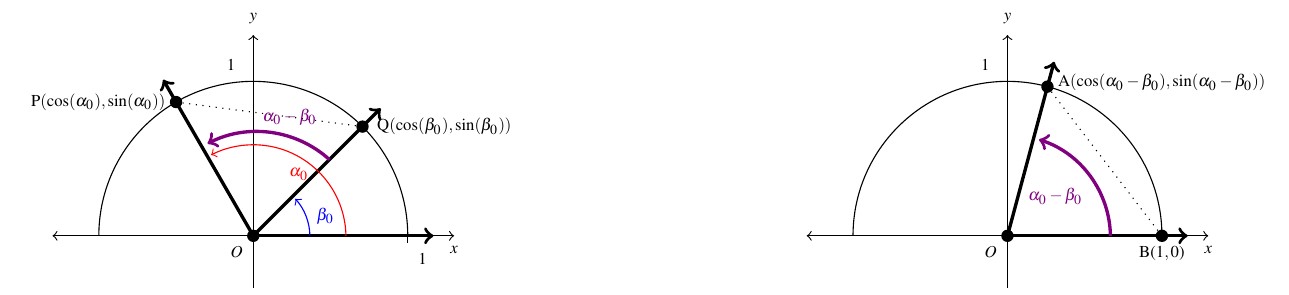
Because the angles $POQ$ and $AOB$ are congruent, the distance between $P$ and $Q$ is equal to the distance between $A$ and $B$ .^[1] The distance formula, Equation 1.1, yields

$\begin{array}{rcl} \sqrt{(\cos(\alpha_{0}) - \cos(\beta_{0}))^2 + (\sin(\alpha_{0}) - \sin(\beta_{0}))^2 } & = & \sqrt{(\cos(0} - \beta_{0}) - 1)^2 + (\sin(\alpha_{0} - \beta_{0}) - 0)^2} \\ \end{array}$

Squaring both sides, we expand the left hand side of this equation as

$\begin{array}{rcl} (\cos(\alpha_{0}) - \cos(\beta_{0}))^2 + (\sin(\alpha_{0}) - \sin(\beta_{0}))^2 & = & \cos^2(\alpha_{0}) - 2\cos(\alpha_{0})\cos(\beta_{0}) + \cos^2(\beta_{0}) \\ & & + \sin^2(\alpha_{0}) - 2\sin(\alpha_{0})\sin(\beta_{0}) + \sin^2(\beta_{0}) \\ [6pt] & = & \cos^2(\alpha_{0}) + \sin^2(\alpha_{0}) + \cos^2(\beta_{0}) + \sin^2(\beta_{0}) \\ & & - 2\cos(\alpha_{0})\cos(\beta_{0}) - 2\sin(\alpha_{0})\sin(\beta_{0}) \end{array}$

From the Pythagorean Identities, $\cos^2(\alpha_{0}) + \sin^2(\alpha_{0}) = 1$ and $\cos^2(\beta_{0}) + \sin^2(\beta_{0}) = 1$ , so

$\begin{array}{rcl} (\cos(\alpha_{0}) - \cos(\beta_{0}))^2 + (\sin(\alpha_{0}) - \sin(\beta_{0}))^2 & = & 2 - 2\cos(\alpha_{0})\cos(\beta_{0}) - 2\sin(\alpha_{0})\sin(\beta_{0}) \end{array}$

Turning our attention to the right hand side of our equation, we find

$\begin{array}{rcl} (\cos(\alpha_{0} - \beta_{0}) - 1)^2 + (\sin(\alpha_{0} - \beta_{0}) - 0)^2 & = & \cos^2(\alpha_{0} - \beta_{0}) - 2\cos(\alpha_{0} - \beta_{0}) + 1 + \sin^2(\alpha_{0} - \beta_{0}) \\ & = & 1 + \cos^2(\alpha_{0} - \beta_{0}) + \sin^2(\alpha_{0} - \beta_{0}) - 2\cos(\alpha_{0} - \beta_{0}) \\ \end{array}$

Once again, we simplify $\cos^2(\alpha_{0} - \beta_{0}) + \sin^2(\alpha_{0} - \beta_{0})= 1$ , so that

$\begin{array}{rcl} (\cos(\alpha_{0} - \beta_{0}) - 1)^2 + (\sin(\alpha_{0} - \beta_{0}) - 0)^2 & = & 2 - 2\cos(\alpha_{0} - \beta_{0}) \\ \end{array}$

Putting it all together, we get $2 - 2\cos(\alpha_{0})\cos(\beta_{0}) - 2\sin(\alpha_{0})\sin(\beta_{0}) = 2 - 2\cos(\alpha_{0} - \beta_{0})$ , which simplifies to: $\cos(\alpha_{0} - \beta_{0}) = \cos(\alpha_{0})\cos(\beta_{0}) + \sin(\alpha_{0})\sin(\beta_{0})$ .

Given $\alpha$ and $\alpha_{0}$ , $\beta$ and $\beta_{0}$ , and $(\alpha - \beta)$ and $(\alpha_{0}- \beta_{0})$ are all coterminal pairs of angles, we have established the identity: $\cos(\alpha - \beta) = \cos(\alpha) \cos(\beta) + \sin(\alpha) \sin(\beta)$ .

For the case where $\alpha_{0} \leq \beta_{0}$ , we can apply the above argument to the angle $\beta_{0} - \alpha_{0}$ to obtain the identity $\cos(\beta_{0} - \alpha_{0}) = \cos(\beta_{0})\cos(\alpha_{0}) + \sin(\beta_{0})\sin(\alpha_{0})$ . Using this formula in conjunction with the Even Identity of cosine gives us the result in this case, too:

$\begin{array}{rcl} \cos(\alpha_{0} - \beta_{0}) = \cos( - (\alpha_{0} - \beta_{0})) = \cos(\beta_{0} - \alpha_{0}) & = & \cos(\beta_{0})\cos(\alpha_{0}) + \sin(\beta_{0})\sin(\alpha_{0}) \\ & = & \cos(\alpha_{0})\cos(\beta_{0}) + \sin(\alpha_{0})\sin(\beta_{0}). \end{array}$

To get the sum identity for cosine, we use the difference formula along with the Even/Odd Identities

$\cos(\alpha + \beta) = \cos(\alpha - (-\beta)) = \cos(\alpha) \cos(-\beta) + \sin(\alpha) \sin(-\beta) = \cos(\alpha) \cos(\beta) - \sin(\alpha) \sin(\beta).$

We put these newfound identities to good use in the following example.

Example 8.2.1

Example 8.2.1.1

Compute the exact value of $\cos\left(15^{\circ}\right)$ .

Solution:

Compute the exact value of $\cos\left(15^{\circ}\right).$

In order to use Theorem 8.5 to find $\cos\left(15^{\circ}\right)$ , we need to write $15^{\circ}$ as a sum or difference of angles whose cosines and sines we know. One way to do so is to write $15^{\circ} = 45^{\circ} - 30^{\circ}$ . We find:

$\begin{array}{rcl} \cos\left(15^{\circ}\right) & = & \cos\left(45^{\circ} - 30^{\circ} \right) \\ [2pt] & = & \cos\left(45^{\circ}\right)\cos\left(30^{\circ} \right) + \sin\left(45^{\circ}\right)\sin\left(30^{\circ} \right) \\ [2pt] & = & \left( \dfrac{\sqrt{2}}{2} \right)\left( \dfrac{\sqrt{3}}{2} \right) + \left( \dfrac{\sqrt{2}}{2} \right)\left( \dfrac{1}{2} \right)\\ [15pt] & = & \dfrac{\sqrt{6}+ \sqrt{2}}{4}. \\ \end{array}$

Example 8.2.1.2

Verify the identity: $\cos\left(\frac{\pi}{2} - \theta\right) = \sin(\theta)$ .

Solution:

Verify the identity: $\cos\left(\frac{\pi}{2} - \theta\right) = \sin(\theta).$

Using Theorem 8.5 gives:

$\begin{array}{rcl} \cos\left(\dfrac{\pi}{2} - \theta\right) & = & \cos\left(\dfrac{\pi}{2}\right)\cos\left(\theta\right) + \sin\left(\dfrac{\pi}{2}\right)\sin\left(\theta \right) \\ [10pt] & = & \left( 0 \right)\left( \cos(\theta) \right) + \left( 1 \right)\left( \sin(\theta) \right) \\ [4pt] & = & \sin(\theta) . \\ \end{array}$

Example 8.2.1.3

Suppose $\alpha$ is a Quadrant I angle with $\sin(\alpha) = \frac{3}{5}$ and $\beta$ is a Quadrant IV angle with $\sec(\beta) = 4$ . Determine the exact value of $\cos(\alpha + \beta)$ .

Solution:

Suppose $\alpha$ is a Quadrant I angle with $\sin(\alpha) = \frac{3}{5}$ and $\beta$ is a Quadrant IV angle with $\sec(\beta) = 4$ . Determine the exact value of $\cos(\alpha + \beta).$

Per Theorem 8.5, we know $\cos(\alpha + \beta) = \cos(\alpha) \cos(\beta) - \sin(\alpha) \sin(\beta)$ . Hence, we need to find the sines and cosines of $\alpha$ and $\beta$ to complete the problem.

We are given $\sin(\alpha) = \frac{3}{5}$ , so our first task is to find $\cos(\alpha)$ . We can quickly get $\cos(\alpha)$ using the Pythagorean Identity $\cos^{2}(\alpha) = 1 - \sin^{2}(\alpha) = 1 - \left(\frac{3}{5}\right)^2 = \frac{16}{25}$ . We get $\cos(\alpha) = \frac{4}{5}$ , choosing the positive root because $\alpha$ is a Quadrant I angle.

Next, we need the $\sin(\beta)$ and $\cos(\beta)$ . $\sec(\beta) = 4$ , so we immediately get $\cos(\beta) = \frac{1}{4}$ courtesy of the Reciprocal and Quotient Identities.

To get $\sin(\beta)$ , we employ the Pythagorean Identity: $\sin^{2}(\beta) = 1 - \cos^{2}(\beta) = 1 - \left(\frac{1}{4} \right)^2 = \frac{15}{16}.$ Here, as $\beta$ is a Quadrant IV angle, we get $\sin(\beta) = - \frac{\sqrt{15}}{4}.$

Finally, we get:

$\begin{array}{rcl} \cos(\alpha + \beta) &=& \cos(\alpha) \cos(\beta) - \sin(\alpha) \sin(\beta) \\[4pt] &=& \left( \frac{4}{5} \right) \left( \frac{1}{4} \right) - \left( \frac{3}{5} \right) \left( - \frac{\sqrt{15}}{4} \right)\\[4pt] &=& \frac{4+3\sqrt{15}}{20} \end{array}$

The identity verified in Example 8.2.1, namely, $\cos\left(\frac{\pi}{2} - \theta\right) = \sin(\theta)$ , is the first of the celebrated `cofunction’ identities.

From $\sin(\theta) = \cos\left(\frac{\pi}{2} - \theta\right)$ , we get: $\sin\left(\frac{\pi}{2} - \theta\right) = \cos\left(\frac{\pi}{2} -\left[\frac{\pi}{2} - \theta\right]\right) = \cos(\theta)$ , which says, in words, that the `co’sine of an angle is the sine of its `co’mplement. Now that these identities have been established for cosine and sine, the remaining circular functions follow suit. The remaining proofs are left as exercises.

Theorem 8.6 Cofunction Identities

For all applicable angles $\theta$ ,

$\cos\left(\dfrac{\pi}{2} - \theta \right) = \sin(\theta)$
$\sin\left(\dfrac{\pi}{2} - \theta \right) = \cos(\theta)$
$\sec\left(\dfrac{\pi}{2} - \theta \right) = \csc(\theta)$
$\csc\left(\dfrac{\pi}{2} - \theta \right) = \sec(\theta)$
$\tan\left(\dfrac{\pi}{2} - \theta \right) = \cot(\theta)$
$\cot\left(\dfrac{\pi}{2} - \theta \right) = \tan(\theta)$

The Cofunction Identities enable us to derive the sum and difference formulas for sine. We first convert to sine to cosine and expand:

$\begin{array}{rcl} \sin(\alpha + \beta) & = & \cos\left( \dfrac{\pi}{2} - (\alpha + \beta) \right) \\ [10pt] & = & \cos\left( \left[\dfrac{\pi}{2} - \alpha \right] - \beta \right) \\ [10pt] & = & \cos\left(\dfrac{\pi}{2} - \alpha \right) \cos(\beta) + \sin\left(\dfrac{\pi}{2} - \alpha \right)\sin(\beta) \\ [10pt] & = & \sin(\alpha) \cos(\beta) + \cos(\alpha) \sin(\beta) \\ \end{array}$

We can derive the difference formula for sine by rewriting $\sin(\alpha - \beta)$ as $\sin(\alpha + (-\beta))$ and using the sum formula and the Even / Odd Identities. Again, we leave the details to the reader.

Theorem 8.7 Sum and Difference Identities for Sine

For all angles $\alpha$ and $\beta$ ,

$\sin(\alpha + \beta) = \sin(\alpha) \cos(\beta) + \cos(\alpha) \sin(\beta)$
$\sin(\alpha - \beta) = \sin(\alpha) \cos(\beta) - \cos(\alpha) \sin(\beta)$

We try out these new identities in the next example.

Example 8.2.2

Example 8.2.2.1

Compute the exact value of $\sin\left(\frac{19 \pi}{12}\right)$

Solution:

Compute the exact value of $\sin\left(\frac{19 \pi}{12}\right).$

As in Example 8.2.1, we need to write the angle $\frac{19 \pi}{12}$ as a sum or difference of common angles. The denominator of $12$ suggests a combination of angles with denominators $3$ and $4$ . One such combination^[2] is $\; \frac{19 \pi}{12} = \frac{4 \pi}{3} + \frac{\pi}{4}$ . Applying Theorem 8.7, we get

$\begin{array}{rcl} \sin\left(\dfrac{19 \pi}{12}\right) & = & \sin\left(\dfrac{4 \pi}{3} + \dfrac{\pi}{4} \right) \\ [10pt] & = & \sin\left(\dfrac{4 \pi}{3} \right)\cos\left(\dfrac{\pi}{4} \right) + \cos\left(\dfrac{4 \pi}{3} \right)\sin\left(\dfrac{\pi}{4} \right) \\ [10pt] & = & \left( -\dfrac{\sqrt{3}}{2} \right)\left( \dfrac{\sqrt{2}}{2} \right) + \left( -\dfrac{1}{2} \right)\left( \dfrac{\sqrt{2}}{2} \right) \\ [15pt] & = & \dfrac{-\sqrt{6}- \sqrt{2}}{4} \\ \end{array}$

Example 8.2.2.2

Suppose $\alpha$ is a Quadrant II angle with $\sin(\alpha) = \frac{5}{13}$ , and $\beta$ is a Quadrant III angle with $\tan(\beta) = 2$ . Compute the exact value of $\sin(\alpha - \beta)$ .

Solution:

Suppose $\alpha$ is a Quadrant II angle with $\sin(\alpha) = \frac{5}{13}$ , and $\beta$ is a Quadrant III angle with $\tan(\beta) = 2$ . Compute the exact value of $\sin(\alpha - \beta)$ .

In order to find $\sin(\alpha - \beta)$ using Theorem 8.7, we need to find $\cos(\alpha)$ and both $\cos(\beta)$ and $\sin(\beta)$ .

To find $\cos(\alpha)$ , we use the Pythagorean Identity $\cos^2(\alpha) = 1 - \sin^{2}(\alpha) = 1 - \left(\frac{5}{13}\right)^2 = \frac{144}{169}$ . We get $\cos(\alpha) = -\frac{12}{13}$ , the negative, here, owing to the fact that $\alpha$ is a Quadrant II angle.

We now set about finding $\sin(\beta)$ and $\cos(\beta)$ . We have several ways to proceed at this point, but as there isn’t a direct way to get from $\tan(\beta) = 2$ to either $\sin(\beta)$ or $\cos(\beta)$ , we opt for a more geometric approach as presented in Section 7.4.

Because $\beta$ is a Quadrant III angle with $\tan(\beta) = 2 = \frac{-2}{-1}$ , we know the point $Q(x,y) = (-1,-2)$ is on the terminal side of $\beta$ as illustrated.^[3]

Rendered by QuickLaTeX.com

We find $r = \sqrt{x^2 + y^2} = \sqrt{(-1)^2+(-2)^2} = \sqrt{5}$ , so per Theorem 7.10, $\sin(\beta) = \frac{-2}{\sqrt{5}} = - \frac{2\sqrt{5}}{5}$ and $\cos(\beta) = \frac{-1}{\sqrt{5}} = - \frac{\sqrt{5}}{5}.$

At last, we have

$\begin{array}{rcl} \sin(\alpha - \beta) &=& \sin(\alpha)\cos(\beta) - \cos(\alpha)\sin(\beta)\\[4pt] &=& \left( \frac{5}{13} \right)\left( -\frac{\sqrt{5}}{5} \right) - \left( -\frac{12}{13} \right)\left( - \frac{2 \sqrt{5}}{5} \right)\\[4pt] &=& -\frac{29\sqrt{5}}{65} \end{array}$

Example 8.2.2.3

Derive a formula for $\tan(\alpha + \beta)$ in terms of $\tan(\alpha)$ and $\tan(\beta)$ .

Solution:

Derive a formula for $\tan(\alpha + \beta)$ in terms of $\tan(\alpha)$ and $\tan(\beta)$ .
We can start by expanding $\tan(\alpha + \beta)$ using a quotient identity and then the sum formulas

$\begin{array}{rcl} \tan(\alpha + \beta) & = & \dfrac{\sin(\alpha + \beta)}{\cos(\alpha + \beta)} \\ [10pt] & = & \dfrac{\sin(\alpha) \cos(\beta) + \cos(\alpha) \sin(\beta)}{\cos(\alpha) \cos(\beta) - \sin(\alpha) \sin(\beta)} \\ \end{array}$

As $\tan(\alpha) = \frac{\sin(\alpha)}{\cos(\alpha)}$ and $\tan(\beta) = \frac{\sin(\beta)}{\cos(\beta)}$ , it looks as though if we divide both numerator and denominator by $\cos(\alpha) \cos(\beta)$ we will have what we want

$\begin{array}{rcl} \tan(\alpha + \beta) & = & \dfrac{\sin(\alpha) \cos(\beta) + \cos(\alpha) \sin(\beta)}{\cos(\alpha) \cos(\beta) - \sin(\alpha) \sin(\beta)} \cdot\dfrac{\dfrac{1}{\cos(\alpha) \cos(\beta)}}{\dfrac{1}{\cos(\alpha) \cos(\beta)}}\\ & & \\ & = & \dfrac{\dfrac{\sin(\alpha) \cos(\beta)}{\cos(\alpha) \cos(\beta)} + \dfrac{\cos(\alpha) \sin(\beta)}{\cos(\alpha) \cos(\beta)}}{\dfrac{\cos(\alpha) \cos(\beta)}{\cos(\alpha) \cos(\beta)} - \dfrac{\sin(\alpha) \sin(\beta)}{\cos(\alpha) \cos(\beta)}}\\ & & \\ & = & \dfrac{\dfrac{\sin(\alpha) \cancel{\cos(\beta)}}{\cos(\alpha) \cancel{\cos(\beta)}} + \dfrac{\cancel{\cos(\alpha)} \sin(\beta)}{\cancel{\cos(\alpha)} \cos(\beta)}}{\dfrac{\cancel{\cos(\alpha)} \cancel{\cos(\beta)}}{\cancel{\cos(\alpha)} \cancel{\cos(\beta)}} - \dfrac{\sin(\alpha) \sin(\beta)}{\cos(\alpha) \cos(\beta)}}\\ & & \\ & = & \dfrac{\tan(\alpha) + \tan(\beta)}{1 -\tan(\alpha) \tan(\beta)} \\[-1em] \end{array}$

Naturally, this formula is limited to those cases where all of the tangents are defined.

The formula developed in Exercise 8.2.2 for $\tan(\alpha + \beta)$ can be used to find a formula for $\tan(\alpha - \beta)$ by rewriting the difference as a sum, $\tan(\alpha + (-\beta))$ and using the odd property of tangent. (The reader is encouraged to fill in the details.) Below we summarize all of the sum and difference formulas.

Theorem 8.8 Sum and Difference Identities

For all applicable angles $\alpha$ and $\beta$ ,

$\cos(\alpha \pm \beta) = \cos(\alpha) \cos(\beta) \mp \sin(\alpha) \sin(\beta)$
$\sin(\alpha \pm \beta) = \sin(\alpha) \cos(\beta) \pm \cos(\alpha) \sin(\beta)$
$\tan(\alpha \pm \beta) = \dfrac{\tan(\alpha) \pm \tan(\beta)}{1 \mp \tan(\alpha) \tan(\beta)}$

In the statement of Theorem 8.8, we have combined the cases for the sum ` $+$ ‘ and difference ` $-$ ‘ of angles into one formula. The convention here is that if you want the formula for the sum ` $+$ ‘ of two angles, you use the top sign in the formula; for the difference, ` $-$ ‘, use the bottom sign. For example,

$\tan(\alpha - \beta) = \dfrac{\tan(\alpha) - \tan(\beta)}{1 + \tan(\alpha) \tan(\beta)}$

If we set $\alpha = \beta$ in the sum formulas in Theorem 8.8, we obtain the following `Double Angle’ Identities:

Theorem 8.9 Double Angle Identities

For all applicable angles $\theta$ ,

$\cos(2\theta) = \left\{ \begin{array}{l} \cos^{2}(\theta) - \sin^{2}(\theta)\\ [5pt] 2\cos^{2}(\theta) - 1 \\ [5pt] 1-2\sin^{2}(\theta) \end{array} \right.$
$\sin(2\theta) = 2\sin(\theta)\cos(\theta)$
$\tan(2\theta) = \dfrac{2\tan(\theta)}{1 - \tan^{2}(\theta)}$

The three different forms for $\cos(2\theta)$ can be explained by our ability to `exchange’ squares of cosine and sine via the Pythagorean Identity. For instance, if we substitute $\sin^{2}(\theta) = 1 - \cos^{2}(\theta)$ into the first formula for $\cos(2\theta)$ , we get $\cos(2\theta) = \cos^{2}(\theta) - \sin^{2}(\theta) = \cos^{2}(\theta) - (1 - \cos^{2}(\theta)) = 2 \cos^{2}(\theta) - 1$ .

It is interesting to note that to determine the value of $\cos(2\theta)$ , only one piece of information is required: either $\cos(\theta)$ or $\sin(\theta)$ . To determine $\sin(2\theta)$ , however, it appears that we must know both $\sin(\theta)$ and $\cos(\theta)$ . In the next example, we show how we can find $\sin(2\theta)$ knowing just one piece of information, namely $\tan(\theta).$

Example 8.2.3

Example 8.2.3.1

Suppose $P(-3,4)$ lies on the terminal side of $\theta$ when $\theta$ is plotted in standard position.

Compute $\cos(2\theta)$ and $\sin(2\theta)$ and determine the quadrant in which the terminal side of the angle $2\theta$ lies when it is plotted in standard position.

Solution:

Suppose $P(-3,4)$ lies on the terminal side of $\theta$ when $\theta$ is plotted in standard position. Compute $\cos(2\theta)$ and $\sin(2\theta)$ .

We sketch the terminal side of $\theta$ below. Using Theorem 7.4 from Section 7.2.2 with $x = -3$ and $y=4$ , we find $r = \sqrt{x^2+y^2} = 5$ . Hence, $\cos(\theta) = -\frac{3}{5}$ and $\sin(\theta) = \frac{4}{5}$ .

Rendered by QuickLaTeX.com

Theorem 8.9 gives us three different formulas to choose from to find $\cos(2\theta)$ . Using the first formula,^[4] we get:

$\begin{array}{rcl} \cos(2\theta) &=& \cos^{2}(\theta) - \sin^{2}(\theta) \\[4pt] &=& \left(-\frac{3}{5}\right)^2 - \left(\frac{4}{5}\right)^2 \\[4pt] &=& -\frac{7}{25} \end{array}$

For $\sin(2\theta)$ , we get

$\begin{array}{rcl} \sin(2\theta) &=& 2 \sin(\theta) \cos(\theta) \\[4pt] &=& 2 \left(\frac{4}{5}\right)\left(-\frac{3}{5}\right) \\[4pt] &=& -\frac{24}{25} \end{array}$

Both cosine and sine of $2\theta$ are negative, the terminal side of $2\theta$ , when plotted in standard position, lies in Quadrant III. To see this more clearly, we plot the terminal side of $2\theta$ , along with the terminal side of $\theta$ .

Rendered by QuickLaTeX.com

Note that in order to find the point $Q(x,y)$ on the terminal side of $2\theta$ of a circle of radius $5$ , we use Theorem 7.4 again and find

$x = r \cos(2\theta) = 5 \left(-\frac{7}{25} \right) = -\frac{7}{5} \text{ and } y = r \sin(2\theta) = 5 \left(-\frac{24}{25}\right) = -\frac{24}{5}$

Example 8.2.3.2

If $\sin(\theta) = x$ for $-\frac{\pi}{2} \leq \theta \leq \frac{\pi}{2}$ , find an expression for $\sin(2\theta)$ in terms of $x$ .

Solution:

If $\sin(\theta) = x$ for $-\frac{\pi}{2} \leq \theta \leq \frac{\pi}{2}$ , find an expression for $\sin(2\theta)$ in terms of $x$ .

If your first reaction to ` $\sin(\theta) = x$ ‘ is `No it’s not, $\cos(\theta) = x$ !’ then you have indeed learned something, and we take comfort in that.

While we have mostly used ` $x$ ‘ to represent the $x$ -coordinate of the point the terminal side of an angle $\theta$ , here, ` $x$ ‘ represents the quantity $\sin(\theta)$ and our task is to express $\sin(2\theta)$ in terms of $x$ .

As a result of $\sin(2\theta) = 2 \sin(\theta) \cos(\theta) = 2 x \cos(\theta)$ , what remains is to express $\cos(\theta)$ in terms of $x$ .

Substituting $\sin(\theta) = x$ into the Pythagorean Identity, we get $\cos^{2}(\theta) = 1- \sin^{2}(\theta) = 1 - x^2$ , or $\cos(\theta) = \pm \sqrt{1-x^2}$ . Given $-\frac{\pi}{2} \leq \theta \leq \frac{\pi}{2}$ , $\cos(\theta) \geq 0$ , and thus $\cos(\theta) = \sqrt{1-x^2}$ .

Our final answer is $\sin(2\theta) = 2 \sin(\theta) \cos(\theta) = 2x\sqrt{1-x^2}$ .

Example 8.2.3.3

Verify the identity: $\sin(2\theta) = \dfrac{2\tan(\theta)}{1 + \tan^{2}(\theta)}$ .

Solution:

Verify the identity: $\sin(2\theta) = \dfrac{2\tan(\theta)}{1 + \tan^{2}(\theta)}$ .

We start with the right hand side of the identity and note that $1 + \tan^{2}(\theta) = \sec^{2}(\theta)$ . Next, we use the Reciprocal and Quotient Identities to rewrite $\tan(\theta)$ and $\sec(\theta)$ in terms of $\sin(\theta)$ and $\cos(\theta)$ :

$\begin{array}{rcl} \dfrac{2\tan(\theta)}{1 + \tan^{2}(\theta)} & = & \dfrac{2\tan(\theta)}{\sec^{2}(\theta)} \\[0.25in] &=& \dfrac{2 \left( \dfrac{\sin(\theta)}{\cos(\theta)}\right)}{\dfrac{1}{\cos^{2}(\theta)}} \\[0.4in] &=& 2\left( \dfrac{\sin(\theta)}{\cos(\theta)}\right) \cos^{2}(\theta) \\[0.25in] & = & 2\left( \dfrac{\sin(\theta)}{\cancel{\cos(\theta)}}\right) \cancel{\cos(\theta)} \cos(\theta) \\[0.1in] &=& 2\sin(\theta) \cos(\theta) = \sin(2\theta). \end{array}$

Example 8.2.3.4

Express $\cos(3\theta)$ as a polynomial in terms of $\cos(\theta).$

Solution:

Express $\cos(3\theta)$ as a polynomial in terms of $\cos(\theta)$ .

In Theorem 8.9, one of the formulas for $\cos(2\theta)$ , namely $\cos(2\theta) = 2\cos^{2}(\theta) - 1$ , expresses $\cos(2\theta)$ as a polynomial in terms of $\cos(\theta)$ . We are now asked to find such an identity for $\cos(3\theta)$ .

Using the sum formula for cosine, we begin with

$\begin{array}{rcl} \cos(3\theta) & = & \cos(2\theta + \theta) \\ [2pt] & = & \cos(2\theta)\cos(\theta) - \sin(2\theta)\sin(\theta). \\ \end{array}$

Our ultimate goal is to express the right hand side in terms of $\cos(\theta)$ only. To that end, we substitute $\cos(2\theta) = 2\cos^{2}(\theta) -1$ and $\sin(2\theta) = 2\sin(\theta)\cos(\theta)$ which yields:

$\begin{array}{rcl} \cos(3\theta) & = & \cos(2\theta)\cos(\theta) - \sin(2\theta)\sin(\theta) \\ [2pt] & = & \left(2\cos^{2}(\theta) - 1\right) \cos(\theta) - \left(2 \sin(\theta) \cos(\theta) \right)\sin(\theta) \\ [2pt] & = & 2\cos^{3}(\theta)- \cos(\theta) - 2 \sin^2(\theta) \cos(\theta) \\ \end{array}$

Finally, we exchange $\sin^{2}(\theta) = 1 - \cos^{2}(\theta)$ courtesy of the Pythagorean Identity, and get

$\begin{array}{rcl} \cos(3\theta) & = & 2\cos^{3}(\theta)- \cos(\theta) - 2 \sin^2(\theta) \cos(\theta) \\ [2pt] & = & 2\cos^{3}(\theta)- \cos(\theta) - 2 \left(1 - \cos^{2}(\theta)\right) \cos(\theta) \\ [2pt] & = & 2\cos^{3}(\theta)- \cos(\theta) - 2\cos(\theta) + 2\cos^{3}(\theta) \\ [2pt] & = & 4\cos^{3}(\theta)- 3\cos(\theta). \\ \end{array}$

Hence, $\cos(3\theta) = 4\cos^{3}(\theta)- 3\cos(\theta)$ .

In the last problem in Example 8.2.3, we saw how we could rewrite $\cos(3\theta)$ as sums of powers of $\cos(\theta)$ . In Calculus, we have occasion to do the reverse; that is, reduce the power of cosine and sine.

Solving the identity $\cos(2\theta) = 2\cos^{2}(\theta) -1$ for $\cos^{2}(\theta)$ and the identity $\cos(2\theta) = 1 - 2\sin^{2}(\theta)$ for $\sin^{2}(\theta)$ results in the aptly-named `Power Reduction’ formulas below.

Theorem 8.10 Power Reduction Formulas

For all angles $\theta$ ,

$\cos^{2}(\theta) = \dfrac{1 + \cos(2\theta)}{2}$
$\sin^{2}(\theta) = \dfrac{1 - \cos(2\theta)}{2}$

Our next example is a typical application of Theorem 8.10 that you’ll likely see in Calculus.

Example 8.2.4

Rewrite $\sin^{2}(\theta) \cos^{2}(\theta)$ as a sum and difference of cosines to the first power.

Solution:

We begin with a straightforward application of Theorem 8.10

$\begin{array}{rcl} \sin^{2}(\theta) \cos^{2}(\theta) & = & \left( \dfrac{1 - \cos(2\theta)}{2} \right) \left( \dfrac{1 + \cos(2\theta)}{2} \right) \\ [10pt] & = & \dfrac{1}{4}\left(1 - \cos^{2}(2\theta)\right) \\ [10pt] & = & \dfrac{1}{4} - \dfrac{1}{4}\cos^{2}(2\theta) \\ \end{array}$

Next, we apply the power reduction formula to $\cos^{2}(2\theta)$ to finish the reduction

$\begin{array}{rcl} \sin^{2}(\theta) \cos^{2}(\theta) & = & \dfrac{1}{4} - \dfrac{1}{4}\cos^{2}(2\theta) \\ [10pt] & = & \dfrac{1}{4} - \dfrac{1}{4} \left(\dfrac{1 + \cos(2(2\theta))}{2}\right) \\ [10pt] & = & \dfrac{1}{4} - \dfrac{1}{8} - \dfrac{1}{8}\cos(4\theta) \\ [10pt] & = & \dfrac{1}{8} - \dfrac{1}{8}\cos(4\theta) \\ \end{array}$

Another application of the Power Reduction Formulas is the Half Angle Formulas. To start, we apply the Power Reduction Formula to $\cos^{2}\left(\frac{\theta}{2}\right)$

$\cos^{2}\left(\dfrac{\theta}{2}\right) = \dfrac{1 + \cos\left(2 \left(\frac{\theta}{2}\right)\right)}{2} = \dfrac{1 + \cos(\theta)}{2}.$

We can obtain a formula for $\cos\left(\frac{\theta}{2}\right)$ by extracting square roots. In a similar fashion, we may obtain a half angle formula for sine, and by using a quotient formula, obtain a half angle formula for tangent.

We summarize these formulas below.

Theorem 8.11 Half Angle Formulas

For all applicable angles $\theta$ ,

$\cos\left(\dfrac{\theta}{2}\right) = \pm \sqrt{\dfrac{1 + \cos(\theta)}{2}}$
$\sin\left(\dfrac{\theta}{2}\right) = \pm \sqrt{\dfrac{1 - \cos(\theta)}{2}}$
$\tan\left(\dfrac{\theta}{2}\right) = \pm \sqrt{\dfrac{1 - \cos(\theta)}{1+\cos(\theta)}}$

where the choice of $\pm$ depends on the quadrant in which the terminal side of $\dfrac{\theta}{2}$ lies.

Example 8.2.5

Example 8.2.5.1

Use a half angle formula to compute the exact value of $\cos\left(15^{\circ}\right)$ .

Solution:

Use a half angle formula to compute the exact value of $\cos\left(15^{\circ}\right)$ .

To use the half angle formula, we note that $15^{\circ} = \frac{30^{\circ}}{2}$ and $15^{\circ}$ is a Quadrant I angle, so its cosine is positive. Thus we have

$\begin{array}{rcl} \cos\left(15^{\circ}\right) & = & + \sqrt{\dfrac{1+\cos\left(30^{\circ}\right)}{2}} \\[10pt] &=& \sqrt{\dfrac{1+\frac{\sqrt{3}}{2}}{2}}\\ [10pt] & = & \sqrt{\dfrac{1+\frac{\sqrt{3}}{2}}{2}\cdot \dfrac{2}{2}} \\[10pt] &=& \sqrt{\dfrac{2+\sqrt{3}}{4}} = \dfrac{\sqrt{2+\sqrt{3}}}{2} \end{array}$

Back in Example 8.2.1, we found $\cos\left(15^{\circ}\right) = \frac{\sqrt{6}+ \sqrt{2}}{4}$ by using the difference formula for cosine. The reader is encouraged to prove that these two expressions are equal algebraically.

Example 8.2.5.2

Suppose $-\pi \leq t \leq 0$ with $\cos(t) = -\frac{3}{5}$ . Determine $\sin\left(\frac{t}{2}\right)$ .

Solution:

Suppose $-\pi \leq t \leq 0$ with $\cos(t) = -\frac{3}{5}$ . Determine $\sin\left(\frac{t}{2}\right)$ .

If $-\pi \leq t \leq 0$ , then $-\frac{\pi}{2} \leq \frac{t}{2} \leq 0$ , which means $\frac{t}{2}$ corresponds to a Quadrant IV angle. Hence, $\sin\left(\frac{t}{2}\right) < 0$ , so we choose the negative root formula from Theorem 8.11:

$\begin{array}{rcl} \sin\left(\dfrac{t}{2} \right) & = & -\sqrt{\dfrac{1-\cos\left(t \right)}{2}} \\[10pt] &=& -\sqrt{\dfrac{1- \left(-\frac{3}{5}\right)}{2}}\\ [10pt] & = & -\sqrt{\dfrac{1 + \frac{3}{5}}{2} \cdot \dfrac{5}{5}} \\[10pt] &=& -\sqrt{\dfrac{8}{10}} \\[10pt] & =& -\dfrac{2\sqrt{5}}{5} \end{array}$

Example 8.2.5.3

Use the identity given in number 3 of Example 8.2.3 to derive the identity

$\tan\left(\dfrac{\theta}{2}\right) = \dfrac{\sin(\theta)}{1+\cos(\theta)}$

Solution:

Use the identity given in number 3 of Example 8.2.3 to derive the identity $\displaystyle{\tan\left(\frac{\theta}{2}\right) = \frac{\sin(\theta)}{1+\cos(\theta)} }$ .

Instead of our usual approach to verifying identities, namely starting with one side of the equation and trying to transform it into the other, we will start with the identity we proved in number 3 of Example 8.2.3 and manipulate it into the identity we are asked to prove.

The identity we are asked to start with is $\; \sin(2\theta) = \frac{2\tan(\theta)}{1 + \tan^{2}(\theta)}$ . If we are to use this to derive an identity for $\tan\left(\frac{\theta}{2}\right)$ , it seems reasonable to proceed by replacing each occurrence of $\theta$ with $\frac{\theta}{2}$

$\begin{array}{rcl} \sin\left(2 \left(\frac{\theta}{2}\right)\right) & = & \dfrac{2\tan\left(\frac{\theta}{2}\right)}{1 + \tan^{2}\left(\frac{\theta}{2}\right)} \\ [15pt] \sin(\theta) & = & \dfrac{2\tan\left(\frac{\theta}{2}\right)}{1 + \tan^{2}\left(\frac{\theta}{2}\right)} \\ \end{array}$

We now have the $\sin(\theta)$ we need, but we somehow need to get a factor of $1+\cos(\theta)$ involved. We substitute $1 + \tan^{2}\left(\frac{\theta}{2}\right) = \sec^{2}\left(\frac{\theta}{2}\right)$ , and continue to manipulate our given identity by converting secants to cosines.

$\begin{array}{rcl} \sin(\theta) & = & \dfrac{2\tan\left(\frac{\theta}{2}\right)}{1 + \tan^{2}\left(\frac{\theta}{2}\right)} \\ [15pt] \sin(\theta) & = & \dfrac{2\tan\left(\frac{\theta}{2}\right)}{\sec^{2}\left(\frac{\theta}{2}\right)} \\ [15pt] \sin(\theta) & = & 2 \tan\left(\frac{\theta}{2}\right) \cos^{2}\left(\frac{\theta}{2}\right) \\ \end{array}$

Finally, we apply a power reduction formula, and then solve for $\tan\left( \frac{\theta}{2} \right)$

$\begin{array}{rcl} \sin(\theta) & = & 2 \tan\left(\frac{\theta}{2}\right) \cos^{2}\left(\frac{\theta}{2}\right) \\ [5pt] \sin(\theta) & = & 2 \tan\left(\frac{\theta}{2}\right) \left(\dfrac{1 + \cos\left(2 \left(\frac{\theta}{2}\right)\right)}{2}\right) \\ [15pt] \sin(\theta) & = & \tan\left(\frac{\theta}{2}\right) \left(1+\cos(\theta) \right) \\ [5pt] \tan\left(\dfrac{\theta}{2}\right) & = & \dfrac{\sin(\theta)}{1+\cos(\theta)} \\ \end{array}$

Our next batch of identities, the Product to Sum Formulas,^[5] are easily verified by expanding each of the right hand sides in accordance with Theorem 8.8 and as you should expect by now we leave the details as exercises. They are of particular use in Calculus, and we list them here for reference.

Theorem 8.12 Product to Sum Formulas

For all angles $\alpha$ and $\beta$ ,

$\cos(\alpha)\cos(\beta) = \frac{1}{2} \left[ \cos(\alpha - \beta) + \cos(\alpha + \beta)\right]$
$\sin(\alpha)\sin(\beta) = \frac{1}{2} \left[ \cos(\alpha - \beta) - \cos(\alpha + \beta)\right]$
$\sin(\alpha)\cos(\beta) = \frac{1}{2} \left[ \sin(\alpha - \beta) + \sin(\alpha + \beta)\right]$

Related to the Product to Sum Formulas are the Sum to Product Formulas, which we will have need of in Section 8.3.2. These are essentially restatements of the Product to Sum Formulas (by re-labeling the arguments of the sine and cosine functions) and as such, their proofs are left as exercises.

Theorem 8.13 Sum to Product Formulas

For all angles $\alpha$ and $\beta$ ,

$\cos(\alpha) + \cos(\beta) = 2 \cos\left( \dfrac{\alpha + \beta}{2}\right)\cos\left( \dfrac{\alpha - \beta}{2}\right)$
$\cos(\alpha) - \cos(\beta) = - 2 \sin\left( \dfrac{\alpha + \beta}{2}\right)\sin\left( \dfrac{\alpha - \beta}{2}\right)$
$\sin(\alpha) \pm \sin(\beta) = 2 \sin\left( \dfrac{\alpha \pm \beta}{2}\right)\cos\left( \dfrac{\alpha \mp \beta}{2}\right)$

Example 8.2.6

Example 8.2.6.1

Write $\; \cos(2\theta)\cos(6\theta) \;$ as a sum.

Solution:

Write $\; \cos(2\theta)\cos(6\theta) \;$ as a sum.

Identifying $\alpha = 2\theta$ and $\beta = 6\theta$ , we find

$\begin{array}{rcl} \cos(2\theta)\cos(6\theta) & = & \frac{1}{2} \left[ \cos(2\theta - 6\theta) + \cos(2\theta + 6\theta)\right]\\ [4pt] & = & \frac{1}{2} \cos(-4\theta) + \frac{1}{2}\cos(8\theta) \\ [4pt] & = & \frac{1}{2} \cos(4\theta) + \frac{1}{2} \cos(8\theta), \end{array}$

where the last equality is courtesy of the even identity for cosine, $\cos(-4\theta) = \cos(4\theta)$ .

Example 8.2.6.2

Write $\; \sin(\theta) - \sin(3\theta) \;$ as a product.

Solution:

Write $\; \sin(\theta) - \sin(3\theta) \;$ as a product.

Identifying $\alpha = \theta$ and $\beta = 3\theta$ yields

$\begin{array}{rcl} \sin(\theta) - \sin(3\theta) & = & 2 \sin\left( \dfrac{\theta - 3\theta}{2}\right)\cos\left( \dfrac{\theta + 3\theta}{2}\right) \\ [2pt] & = & 2 \sin\left( -\theta \right)\cos\left( 2\theta \right) \\ [2pt] & = & -2 \sin\left( \theta \right)\cos\left( 2\theta \right), \\ \end{array}$

where the last equality is courtesy of the odd identity for sine, $\sin(-\theta) = -\sin(\theta)$ .

The reader is reminded that all of the identities presented in this section which regard the circular functions as functions of angles (in radian measure) apply equally well to the circular (trigonometric) functions regarded as functions of real numbers.

8.2.1 Sinusoids, Revisted

We first studied sinusoids in Section 7.3. Using the sum formulas for sine and cosine, we can expand the forms given to us in Theorem 7.7:

$S(t) = A \sin(B t + C) + D = A\sin(B t) \cos(C) + A \cos(B t)\sin(C) + D,$

and

$E(t) = A \cos(B t + C) + D = A\cos(B t) \cos(C) - A \sin(B t) \sin(C) + B.$

As we’ll see in the next example, recognizing these `expanded’ forms of sinusoids allows us to graph functions as sinusoids which, at first glance, don’t appear to fit the forms of either $E(t)$ or $S(t)$ .

Example 8.2.7

Example 8.2.7.1

Consider the function $f(t) = \cos(2t) - \sqrt{3} \sin(2t)$ .

Write a formula for $f(t)$ in the form $E(t) = A \cos(Bt + C) + D$ for $B > 0$ .

Check your answers analytically using identities.

Solution:

Write a formula for $f(t) = \cos(2t) - \sqrt{3} \sin(2t)$ in the form $E(t) = A \cos(Bt + C) + D$ for $B > 0$ .

The key to this problem is to use the expanded forms of the sinusoid formulas and match up corresponding coefficients. We start by equating $f(t) = \cos(2t) - \sqrt{3} \sin(2t)$ with the expanded form of $E(t) = A \cos(Bt + C) + D$ :

$\cos(2t) - \sqrt{3} \sin(2t) = A\cos(B t) \cos(C) - A \sin(Bt) \sin(C) + D$

If we take $B = 2$ and $D = 0$ , we get:

$\cos(2t) - \sqrt{3} \sin(2t) = A\cos(2t) \cos(C) - A \sin(2t)\sin(C)$

To determine $A$ and $C$ , a bit more work is involved. We get started by equating the coefficients of the trigonometric functions on either side of the equation.

On the left hand side, the coefficient of $\cos(2t)$ is $1$ , while on the right hand side, it is $A \cos(C)$ . As this equation is to hold for all real numbers, we must have that $A \cos(C) = 1$ .

Similarly, we find by equating the coefficients of $\sin(2t)$ that $A \sin(C) = \sqrt{3}$ . In conjunction with $A \cos(C) = 1$ , we have a system of two (nonlinear) equations and two unknowns.

As usual, our first task is to reduce this system of two equations and two unknowns to one equation and one unknown. We can temporarily eliminate the dependence on $C$ by using a Pythagorean Identity. From $\cos^{2}(C) + \sin^{2}(C) = 1$ , we multiply through by $A^2$ to get $A^2\cos^{2}(C) + A^2\sin^{2}(C) = A^2$ .

In our case, $A \cos(C) = 1$ and $A \sin(C) = \sqrt{3}$ , hence

$\begin{array}{rcl} A^2 &=& A^2\cos^{2}(C) + A^2\sin^{2}(C) \\[4pt] &=& 1^2 + (\sqrt{3})^2 = 4 \\[4pt] A &=& \pm 2 \end{array}$

We can choose $A = 2$ , and then find $C$ associated with this choice^[6].

Substituting $A=2$ into our two equations, $A \cos(C) = 1$ and $A \sin(C) = \sqrt{3}$ , we get $2\cos(C) = 1$ and $2 \sin(C) = \sqrt{3}$ . After some rearrangement, $\cos(C) = \frac{1}{2}$ and $\sin(C) = \frac{\sqrt{3}}{2}$ . One such angle $C$ which satisfies this criteria is $C = \frac{\pi}{3}$ .

Hence, one way to write $f(t)$ as a sinusoid is $f(t) = 2 \cos\left(2t + \frac{\pi}{3}\right)$ .

We can check our answer using the sum formula for cosine :

$\begin{array}{rcl} f(t) & = & 2 \cos\left(2t + \frac{\pi}{3}\right) \\ [3pt] & = & 2 \left[ \cos(2t) \cos\left(\frac{\pi}{3}\right) - \sin(2t) \sin\left(\frac{\pi}{3}\right) \right]\\ [3pt] & = & 2 \left[ \cos(2t) \left(\frac{1}{2}\right) - \sin(2t) \left(\frac{\sqrt{3}}{2}\right)\right] \\ [3pt] & = & \cos(2t) - \sqrt{3} \sin(2t). \\ \end{array}$

Example 8.2.7.2

Consider the function $f(t) = \cos(2t) - \sqrt{3} \sin(2t)$ .

Write a formula for $f(t)$ in the form $S(t) = A \sin(B t + C) + D$ for $B > 0$ .

Check your answers analytically using identities.

Solution:

Write a formula for $f(t) = \cos(2t) - \sqrt{3} \sin(2t)$ in the form $S(t) = A \sin(B t + C) + D$ for $B > 0$ .

Proceeding as before, we equate $f(t) = \cos(2t) - \sqrt{3} \sin(2t)$ with the expanded form of of the sinusoid $S(t) = A \sin(Bt +C) + D$ to get:

$\cos(2t) - \sqrt{3} \sin(2t) = A\sin(Bt) \cos(C) + A \cos(Bt)\sin(C) + D$

Taking $B= 2$ and $D = 0$ , we get $\cos(2t) - \sqrt{3} \sin(2t) = A\sin(2t) \cos(C) + A \cos(2t)\sin(C)$ . We equate^[7] the coefficients of $\cos(2t)$ on either side and get $A\sin(C) = 1$ and $A\cos(C) = -\sqrt{3}$ .

Using $A^2\cos^{2}(C) + A^2\sin^{2}(C) = A^2$ as before, we get $A = \pm 2$ , and again we choose $A = 2$ .

This means $2 \sin(C) = 1$ , or $\sin(C) = \frac{1}{2}$ , and $2\cos(C) = -\sqrt{3}$ , so $\cos(C) = -\frac{\sqrt{3}}{2}$ . One such angle which meets these criteria is $C = \frac{5\pi}{6}$ .

Hence, we have $f(t) = 2 \sin\left(2t + \frac{5\pi}{6}\right)$ .

Checking our work analytically, we have

$\begin{array}{rcl} f(t) & = & 2 \sin\left(2t + \frac{5\pi}{6}\right) \\ [3pt] & = & 2 \left[ \sin(2t) \cos\left(\frac{5\pi}{6}\right) + \cos(2t) \sin\left(\frac{5\pi}{6}\right) \right]\\ [3pt] & = & 2 \left[ \sin(2t) \left(-\frac{\sqrt{3}}{2}\right) + \cos(2t) \left(\frac{1}{2}\right)\right] \\ [3pt] & = & \cos(2t) - \sqrt{3} \sin(2t) \\[-1.5em] \end{array}$

A couple of remarks about Example 8.2.7 are in order. First, had we chosen $A = -2$ instead of $A = 2$ as we worked through Example 8.2.7, our final answers would have looked different. The reader is encouraged to rework Example 8.2.7 using $A = -2$ to see what these differences are, and then for a challenging exercise, use identities to show that the formulas are all equivalent.^[8]

It is important to note that in order for the technique presented in Example 8.2.7 to fit a function into one of the forms in Theorem 7.7, the frequencies of the sine and cosine terms must match. For example, in the Exercises, you’ll be asked to write $f(t) = 3\sqrt{3}\sin(3t) - 3\cos(3t)$ in the form of $S(t)$ and $C(t)$ above, and because both the sine and cosine terms have frequency $3$ , this is possible.

However, a function such as $f(t) = \sin(t) - \sin(3t)$ cannot be written in the form of $S(t)$ or $C(t)$ . The quickest way to see this is to examine its graph below which is decidedly not a sinusoid. That being said, we can still analyze this curve using identities.

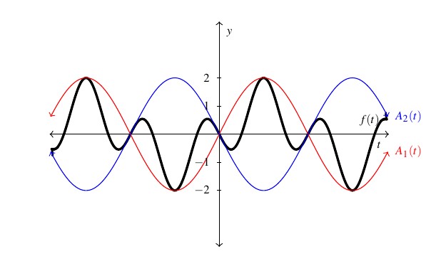
A coordinate plane with two sine of t in red, negative two sine of three t in blue and sine of t minus sine of three t in thick black. — Graph of f(t) Bounded by 2sin(t) and -2sin(t).

Using our result from number 2 Example 8.2.6, we may rewrite $f(t) = \sin(t) - \sin(3t) = -2 \sin(t) \cos(2t)$ . Grouping factors, we can view $f(t) = [ -2 \sin(t) ] \cos(2t) = A(t) \cos(2t)$ as the curve $y = \cos(2t)$ with a variable amplitude, $A(t) = -2 \sin(t)$ .

Overlaying the graphs of $f(t)$ with the (dashed) graphs of $\textcolor{red}{A_{1}(t) = 2 \sin(t)}$ and $\textcolor{blue}{A_{2}(t) = -2 \sin(t)}$ , we can see the role these two curves play in the graph of $y = f(t)$ . They create a kind of `wave envelope’ for the graph of $y = f(t)$ . This is an example of the beats phenomenon. Note that when written as a product of sinusoids, it is always the lower frequency factor which creates the `wave-envelope’ of the curve.

Note that in order to rewrite a sum or difference of sine and cosine functions with different frequencies into a product using the sum to product identities, Theorem 8.13, we need the amplitudes of each term to be the same. We explore more examples of these functions and this behavior in the Exercises.

8.2.2 Section Exercises

In Exercises 1 – 6, use the Even / Odd Identities to verify the identity. Assume all quantities are defined.

$\sin(3\pi - 2\theta) = -\sin(2\theta - 3\pi)$
$\cos \left( -\frac{\pi}{4} - 5t \right) = \cos \left( 5t + \frac{\pi}{4} \right)$
$\tan(-x^{2} + 1) = -\tan(x^{2} - 1)$
$\csc(-\theta - 5) = -\csc(\theta + 5)$
$\sec(-6x) = \sec(6x)$
$\cot(9 - 7\theta) = -\cot(7\theta - 9)$

In Exercises 7 – 21, use the Sum and Difference Identities to find the exact value. You may have need of the Quotient, Reciprocal or Even/Odd Identities as well.

$\cos(75^{\circ})$
$\sec(165^{\circ})$
$\sin(105^{\circ})$
$\csc(195^{\circ})$
$\cot(255^{\circ})$
$\tan(375^{\circ})$
$\cos\left(\frac{13\pi}{12}\right)$
$\sin\left(\frac{11\pi}{12}\right)$
$\tan\left(\frac{13\pi}{12}\right)$
$\cos \left( \frac{7\pi}{12} \right)$
$\tan \left( \frac{17\pi}{12} \right)$
$\sin \left( \frac{\pi}{12} \right)$
$\cot \left( \frac{11\pi}{12} \right)$
$\csc \left( \frac{5\pi}{12} \right)$
$\sec \left( -\frac{\pi}{12} \right)$
If is a Quadrant IV angle with , and , where , find
1. $\cos(\alpha + \beta)$
2. $\sin(\alpha + \beta)$
3. $\tan(\alpha + \beta)$
4. $\cos(\alpha - \beta)$
5. $\sin(\alpha - \beta)$
6. $\tan(\alpha - \beta)$
If , where , and is a Quadrant II angle with , find
1. $\cos(\alpha + \beta)$
2. $\sin(\alpha + \beta)$
3. $\tan(\alpha + \beta)$
4. $\cos(\alpha - \beta)$
5. $\sin(\alpha - \beta)$
6. $\tan(\alpha - \beta)$
If , where , and where , find
1. $\sin(\alpha + \beta)$
2. $\cos(\alpha - \beta)$
3. $\tan(\alpha - \beta)$
If , where , and , where , find
1. $\csc(\alpha - \beta)$
2. $\sec(\alpha + \beta)$
3. $\cot(\alpha + \beta)$

In Exercises 26 – 35, use Example 8.2.7 as a guide to show that the function is a sinusoid by rewriting it in the forms $E(t) = A \cos(B t + C) + D$ and $S(t) = A \sin(Bt + C) + D$ for $B> 0$ and $0 \leq C < 2\pi$ .

$f(t) = \sqrt{2}\sin(t) + \sqrt{2}\cos(t) + 1$
$f(t) = 3\sqrt{3}\sin(3t) - 3\cos(3t)$
$f(t) = -\sin(t) + \cos(t) - 2$
$f(t) = -\frac{1}{2}\sin(2t) - \frac{\sqrt{3}}{2}\cos(2t)$
$f(t) = 2\sqrt{3} \cos(t) - 2\sin(t)$
$f(t) = \frac{3}{2} \cos(2t) - \frac{3\sqrt{3}}{2} \sin(2t) + 6$
$f(t) = -\frac{1}{2} \cos(5t) -\frac{\sqrt{3}}{2} \sin(5t)$
$f(t) = -6\sqrt{3} \cos(3t) - 6\sin(3t) - 3$
$f(t) = \frac{5\sqrt{2}}{2} \sin(t) -\frac{5\sqrt{2}}{2} \cos(t)$
$f(t) =3 \sin \left(\frac{t}{6}\right) -3\sqrt{3} \cos \left(\frac{t}{6}\right)$
In Exercises 26 – 35, you should have noticed a relationship between the phases $C$ for the $S(t)$ and $E(t)$ . Show that if $f(t) = A \sin(Bt + \alpha) + D$ , then $f(t) = A \cos(Bt + \beta) + D$ where $\beta = \alpha - \frac{\pi}{2}$ .
Let $C$ be an angle measured in radians and let $P(a,b)$ be a point on the terminal side of $C$ when it is drawn in standard position. Use Theorem 7.4 and the sum identity for sine in Theorem 8.7 to show that $f(t) = a \, \sin(Bt) + b\, \cos(Bt) + D$ (with $B > 0$ ) can be rewritten as $f(t) = \sqrt{a^{2} + b^{2}}\sin(B t + C) + D$ .
Two (seemingly) different formulas to model the hours of daylight are given here, $H(t)$ : $H_{1}(t) = 9.25 \sin\left(\frac{\pi}{6} t - \frac{\pi}{2}\right) + 12.55$ and $H_{2}(t) = -8.13 \sin\left(\frac{\pi}{6} t - 4.70\right)+ 12.5$ . Use the difference identities for sine to expand $H_{1}(t)$ and $H_{2}(t)$ . How different are they?

In Exercises 39 – 53, verify the identity.^[9]

$\sin\left(\theta + \frac{\pi}{2}\right) = \cos(t)$
$\cos\left(\theta - \frac{\pi}{2} \right) = \sin(t)$
$\cos(\theta - \pi) = -\cos(\theta)$
$\sin(\pi - \theta) = \sin(\theta)$
$\tan\left(\theta + \frac{\pi}{2} \right) = -\cot(\theta)$
$\sin(\alpha + \beta) + \sin(\alpha - \beta) = 2\sin(\alpha)\cos(\beta)$
$\sin(\alpha + \beta) - \sin(\alpha - \beta) = 2\cos(\alpha) \sin(\beta)$
$\cos(\alpha + \beta) + \cos(\alpha - \beta) = 2\cos(\alpha) \cos(\beta)$
$\cos(\alpha + \beta) - \cos(\alpha - \beta) = -2\sin(\alpha) \sin(\beta)$
$\dfrac{\sin(\alpha+\beta)}{\sin(\alpha-\beta)} = \dfrac{1+\cot(\alpha) \tan(\beta)}{1 - \cot(\alpha) \tan(\beta)}$
$\dfrac{\cos(\alpha + \beta)}{\cos(\alpha - \beta)} = \dfrac{1 - \tan(\alpha)\tan(\beta)}{1 + \tan(\alpha)\tan(\beta)}$
$\dfrac{\tan(\alpha + \beta)}{\tan(\alpha - \beta)} = \dfrac{\sin(\alpha)\cos(\alpha) + \sin(\beta)\cos(\beta)}{\sin(\alpha)\cos(\alpha) - \sin(\beta)\cos(\beta)}$
$\dfrac{\sin(t + h) - \sin(t)}{h} = \cos(t) \left(\dfrac{\sin(h)}{h} \right) + \sin(t) \left( \dfrac{\cos(h) - 1}{h} \right)$
$\dfrac{\cos(t + h) - \cos(t)}{h} = \cos(t) \left( \dfrac{\cos(h) - 1}{h} \right) - \sin(t) \left(\dfrac{\sin(h)}{h} \right)$
$\dfrac{\tan(t + h) - \tan(t)}{h} = \left( \dfrac{\tan(h)}{h} \right) \left(\dfrac{\sec^{2}(t)}{1 - \tan(t)\tan(h)} \right)$

In Exercises 54 – 63, use the Half Angle Formulas to find the exact value. You may have need of the Quotient, Reciprocal or Even/Odd Identities as well.

$\cos(75^{\circ})$ (compare with Exercise 7)
$\sin(105^{\circ})$ (compare with Exercise 9)
$\cos(67.5^{\circ})$
$\sin(157.5^{\circ})$
$\tan(112.5^{\circ})$
$\cos\left( \frac{7\pi}{12} \right)$ (compare with Exercise 16)
$\sin\left( \frac{\pi}{12} \right)$ (compare with Exercise 18)
$\cos \left( \frac{\pi}{8} \right)$
$\sin \left( \frac{5\pi}{8} \right)$
$\tan \left( \frac{7\pi}{8} \right)$

In Exercises 64 – 73, use the given information about $\theta$ to compute the exact values of

$\sin(2\theta)$
$\cos(2\theta)$
$\tan(2\theta)$
$\sin\left(\frac{\theta}{2}\right)$
$\cos\left(\frac{\theta}{2}\right)$
$\tan\left(\frac{\theta}{2}\right)$

$\sin(\theta) = -\frac{7}{25}$ where $\frac{3\pi}{2} < \theta < 2\pi$
$\cos(\theta) = \frac{28}{53}$ where $0 < \theta < \frac{\pi}{2}$
$\tan(\theta) = \frac{12}{5}$ where $\pi < \theta < \frac{3\pi}{2}$
$\csc(\theta) = 4$ where $\frac{\pi}{2} < \theta < \pi$
$\cos(\theta) = \frac{3}{5}$ where $0 < \theta < \frac{\pi}{2}$
$\sin(\theta) = -\frac{4}{5}$ where $\pi < \theta < \frac{3\pi}{2}$
$\cos(\theta) = \frac{12}{13}$ where $\frac{3\pi}{2} < \theta < 2\pi$
$\sin(\theta) = \frac{5}{13}$ where $\frac{\pi}{2} < \theta < \pi$
$\sec(\theta) = \sqrt{5}$ where $\frac{3\pi}{2} < \theta < 2\pi$
$\tan(\theta) = -2$ where $\frac{\pi}{2} < \theta < \pi$

In Exercises 74 – 88, verify the identity. Assume all quantities are defined.

$(\cos(\theta) + \sin(\theta))^2 = 1 + \sin(2\theta)$
$(\cos(\theta) - \sin(\theta))^2 = 1 - \sin(2\theta)$
$\tan(2t) = \frac{1}{1-\tan(t)} - \frac{1}{1+\tan(t)}$
$\csc(2\theta) = \frac{\cot(\theta) + \tan(\theta)}{2}$
$8 \sin^{4}(x) = \cos(4x) - 4\cos(2x)+3$
$8 \cos^{4}(x) = \cos(4x) + 4\cos(2x)+3$
$\sin(3\theta) = 3\sin(\theta) - 4\sin^{3}(\theta)$
$\sin(4\theta) = 4\sin(\theta)\cos^{3}(\theta) - 4\sin^{3}(\theta)\cos(\theta)$
$32\sin^{2}(t) \cos^{4}(t) = 2 + \cos(2t) - 2\cos(4t) - \cos(6t)$
$32\sin^{4}(t) \cos^{2}(t) = 2 - \cos(2t) - 2\cos(4t) + \cos(6t)$
$\cos(4\theta) = 8\cos^{4}(\theta) - 8\cos^{2}(\theta) + 1$
$\cos(8\theta) = 128\cos^{8}(\theta)-256\cos^{6}(\theta)+160\cos^{4}(\theta)-32\cos^{2}(\theta)+1$ (HINT: Use the result to 84.)
$\sec(2x) = \dfrac{\cos(x)}{\cos(x) + \sin(x)} + \dfrac{\sin(x)}{\cos(x)-\sin(x)}$
$\dfrac{1}{\cos(\theta) - \sin(\theta)} + \dfrac{1}{\cos(\theta) + \sin(\theta)} = \dfrac{2\cos(\theta)}{\cos(2\theta)}$
$\dfrac{1}{\cos(\theta) - \sin(\theta)} - \dfrac{1}{\cos(\theta) + \sin(\theta)} = \dfrac{2\sin(\theta)}{\cos(2\theta)}$
Suppose is a Quadrant I angle with . Verify the following formulas
1. $\cos(\theta) = \sqrt{1-x^2}$
2. $\sin(2\theta) = 2x\sqrt{1-x^2}$
3. $\cos(2\theta) = 1 - 2x^2$
Discuss with your classmates how each of the formulas, if any, in Exercise 89 change if we change assume $\theta$ is a Quadrant II, III, or IV angle.
Suppose is a Quadrant I angle with . Verify the following formulas
1. $\cos(\theta) = \dfrac{1}{\sqrt{x^2+1}}$
2. $\sin(\theta) = \dfrac{x}{\sqrt{x^2+1}}$
3. $\sin(2\theta) = \dfrac{2x}{x^2+1}$
4. $\cos(2\theta) = \dfrac{1-x^2}{x^2+1}$
Discuss with your classmates how each of the formulas, if any, in Exercise 91 change if we change assume $\theta$ is a Quadrant II, III, or IV angle.
If $\sin(t) = x$ for $-\frac{\pi}{2} < t < \frac{\pi}{2}$ , find an expression for $\tan(t)$ in terms of $x$ .
If $\tan(\theta) = x$ for $-\frac{\pi}{2} < \theta < \frac{\pi}{2}$ , find an expression for $\sec(\theta)$ in terms of $x$ .
If $\sec(\theta) = x$ where $\theta$ is a Quadrant II angle, find an expression for $\tan(\theta)$ in terns of $x$ .
If $\sin(t) = \frac{x}{2}$ for $-\frac{\pi}{2} < t < \frac{\pi}{2}$ , find an expression for $\cos(2t)$ in terms of $x$ .
If $\tan(\theta) = \frac{x}{7}$ for $-\frac{\pi}{2} < \theta < \frac{\pi}{2}$ , find an expression for $\sin(2\theta)$ in terms of $x$ .
If $\sec(t) = \frac{x}{4}$ for $0 < t < \frac{\pi}{2}$ , find an expression for $\ln|\sec(t) + \tan(t)|$ in terms of $x$ .
Show that $\cos^{2}(\theta) - \sin^{2}(\theta) = 2\cos^{2}(\theta) - 1 = 1 - 2\sin^{2}(\theta)$ for all $\theta$ .
Let $\theta$ be a Quadrant III angle with $\cos(\theta) = -\frac{1}{5}$ . Show that this is not enough information to determine the sign of $\sin\left(\frac{\theta}{2}\right)$ by first assuming $3\pi < \theta < \frac{7\pi}{2}$ and then assuming $\pi < \theta < \frac{3\pi}{2}$ and computing $\sin\left(\frac{\theta}{2}\right)$ in both cases.
Without using your calculator, show that $\frac{\sqrt{2 + \sqrt{3}}}{2} = \frac{\sqrt{6} + \sqrt{2}}{4}$ .
In part 4 of Example 8.2.3, we wrote $\cos(3\theta)$ as a polynomial in terms of $\cos(\theta)$ . In Exercise 84, we had you verify an identity which expresses $\cos(4\theta)$ as a polynomial in terms of $\cos(\theta)$ . Can you find a polynomial in terms of $\cos(\theta)$ for $\cos(5\theta)$ ? $\cos(6\theta)$ ? Can you find a pattern so that $\cos(n\theta)$ could be written as a polynomial in cosine for any natural number $n$ ?
In Exercise 80, we has you verify an identity which expresses $\sin(3\theta)$ as a polynomial in terms of $\sin(\theta)$ . Can you do the same for $\sin(5\theta)$ ? What about for $\sin(4\theta)$ ? If not, what goes wrong?

In Exercises 104 – 109, verify the identity by graphing the right and left hand using a graphing utility.

$\sin^{2}(t) + \cos^{2}(t) = 1$
$\sec^{2}(x) - \tan^{2}(x) = 1$
$\cos(t) = \sin\left(\frac{\pi}{2} - t\right)$
$\tan(x+\pi) = \tan(x)$
$\sin(2t) = 2\sin(t)\cos(t)$
$\tan\left(\frac{x}{2}\right) = \frac{\sin(x)}{1+\cos(x)}$

In Exercises 110 – 115, write the given product as a sum. Note: you may need to use an Even/Odd Identity to match the answer provided.

$\cos(3\theta)\cos(5\theta)$
$\sin(2t)\sin(7t)$
$\sin(9x)\cos(x)$
$\cos(2\theta) \cos(6\theta)$
$\sin(3t) \sin(2t)$
$\cos(x) \sin(3x)$

In Exercises 116 – 121, write the given sum as a product. Note: you may need to use an Even/Odd or Cofunction Identity to match the answer provided.

$\cos(3\theta) + \cos(5\theta)$
$\sin(2t) - \sin(7t)$
$\cos(5x) - \cos(6x)$
$\sin(9\theta) - \sin(-\theta)$
$\sin(t) + \cos(t)$
$\cos(x) - \sin(x)$

In Exercises 122 – 125, using the remarks following Example 8.2.7 as a guide, rewrite the given function $f(t)$ as a product of sinusoids. Identify the functions which create the `wave envelope.’ Check your answer by graphing the function along with the `wave-envelope’ using a graphing utility.

$f(t) = \cos(3t) + \cos(5t)$
$f(t) = 3\cos(5t) - 3\cos(6t)$
$f(t) = \frac{1}{2} \sin(9t) + \frac{1}{2} \sin(t)$
$f(t) = \frac{2}{3}\sin(2t) - \frac{2}{3}\sin(7t)$
Verify the Even / Odd Identities for tangent, secant, cosecant and cotangent.
Verify the Cofunction Identities for tangent, secant, cosecant and cotangent.
Verify the Difference Identities for sine and tangent.
Verify the Product to Sum Identities.
Verify the Sum to Product Identities.

In the picture we've drawn, the triangles $POQ$ and $AOB$ are congruent, which is even better. However, $\alpha_{0} - \beta_{0}$ could be $0$ or it could be $\pi$ , neither of which makes a triangle. It could also be larger than $\pi$ , which makes a triangle, just not the one we've drawn. You should think about those three cases. ↵
It takes some trial and error to find this combination. One alternative is to convert to degrees $\ldots$ ↵
Note that even though $\tan(\beta) = \frac{\sin(\beta)}{\cos(\beta)}$ , we cannot take $\sin(\beta)=-2$ and $\cos(\beta) = -1$ . Recall that $\sin(\beta)$ and $\cos(\beta)$ are the $y$ and $x$ coordinates on a specific circle, the Unit Circle. As we'll see shortly, $(-1,-2)$ lies on a circle of $\sqrt{5}$ , so not the Unit Circle. ↵
We invite the reader to check this answer using the other two formulas. ↵
These are also known as the Prosthaphaeresis Formulas and have a rich history. The authors recommend that you conduct some research on them as your schedule allows. ↵
Remember choosing $A=-2$ results in a different but equally correct phase shift. ↵
Be careful here! ↵
The general equations to fit a function of the form $f(x) = a \, \cos(B x) + b \, \sin(B x) + D$ into one of the forms in Theorem 7.7 are explored in Exercise 36. ↵
Note: numbers 39 and 40 are the conversion formulas stated in Theorem 7.6 in Section 7.3. ↵