8.3 Solving Equations Involving Trigonometric Functions

Vanessa Coffelt

8.3 Solving Equations Involving Trigonometric Functions

8.3.1 Solving Equations Using the Inverse Trigonometric Functions

In Sections 7.2.2 and 7.4, we learned how to solve equations like $\sin(\theta) = \frac{1}{2}$ and $\tan(t) = -1$ . In each case, we ultimately appealed to the Unit Circle and relied on the fact that the answers corresponded to a set of `common angles’ listed in Section 7.2.

If, on the other hand, we had been asked to find all angles with $\sin(\theta) = \frac{1}{3}$ or solve $\tan(t) = -2$ for real numbers $t$ , we would have been hard-pressed to do so. With the introduction of the inverse trigonometric functions, however, we are now in a position to solve these equations.

A good parallel to keep in mind is how the square root function can be used to solve certain quadratic equations. The equation $x^2 = 4$ is a lot like $\sin(\theta) = \frac{1}{2}$ in that it has friendly, `common value’ answers $x = \pm 2$ . The equation $x^2 = 7$ , on the other hand, is a lot like $\sin(\theta) = \frac{1}{3}$ . We know there are answers, but we can’t express them using `friendly’ numbers.

To solve $x^2 = 7$ , we make use of the square root function (which is an inverse to $f(x) = x^2$ on a restricted domain) and write our answer as $x = \pm \sqrt{7}$ . We need the $\pm$ to adjust for the fact that $\sqrt{7}$ is defined to be positive only, but we know we have two solutions, one positive and one negative. Using a calculator, we can certainly approximate the values $\pm \sqrt{7}$ , but as far as exact answers go, we leave them as $x = \pm \sqrt{7}$ .

In the same way, we will use the arcsine function (the inverse to the sine function on a restricted domain) to solve $\sin(\theta) = \frac{1}{3}$ . However, we will need to adjust for the fact that there is more than one answer to this equation (infinitely many, in fact!) As it turns out, we will be able to express every solution in terms of $\arcsin\left(\frac{1}{3}\right)$ , as our next example illustrates.

Example 8.3.1

Example 8.3.1.1

Solve the following equations.

Determine all angles $\theta$ for which $\sin(\theta) = \frac{1}{3}$ .

Solution:

Determine all angles $\theta$ for which $\sin(\theta) = \frac{1}{3}$ .

If $\sin(\theta) = \frac{1}{3}$ , then the terminal side of $\theta$ , when plotted in standard position, intersects the Unit Circle at $y = \frac{1}{3}$ . Geometrically, we see that this happens at two places: in Quadrant I and Quadrant II.

If we let $\alpha$ denote the acute solution to the equation, then all the solutions to this equation in Quadrant I are coterminal with $\alpha$ , and $\alpha$ serves as the reference angle for all of the solutions to this equation in Quadrant II as seen next.

Rendered by QuickLaTeX.com

Considering $\frac{1}{3}$ isn’t the sine of any of the `common angles’ we’ve encountered, we use the arcsine functions to express our answers. By definition, there exists a real number $t = \arcsin\left(\frac{1}{3}\right)$ such that $\sin(t) = \frac{1}{3}$ with $0 < t < \frac{\pi}{2}$ .

Hence, $\alpha = \arcsin\left(\frac{1}{3}\right)$ radians is an acute angle with $\sin(\alpha) = \frac{1}{3}$ . Because all of the Quadrant I solutions $\theta$ are all coterminal with $\alpha$ , we get

$\begin{array}{rcl} \theta &=& \alpha + 2\pi k \\[4pt] &=& \arcsin\left(\frac{1}{3}\right) + 2\pi k \text{ for integers } k \end{array}$

Turning our attention to Quadrant II, we get one solution to be $\pi - \alpha$ . Hence, the Quadrant II solutions are

$\begin{array}{rcl} \theta &=& \pi - \alpha + 2\pi k \\[4pt] &=& \pi - \arcsin\left(\frac{1}{3}\right) + 2\pi k \text{ for integers } k \end{array}$

Example 8.3.1.2

Solve the following equations.

Determine all real numbers $t$ for which $\tan(t) = -2$ .

Solution:

Determine all real numbers $t$ for which $\tan(t) = -2$ .

The real number solutions to $\tan(t)=-2$ correspond to angles $\theta$ with $\tan(\theta) = -2$ . Due to the fact that tangent is negative only in Quadrants II and IV, we focus our efforts there.

The real number $t = \arctan(-2)$ satisfies $\tan(t)=-2$ and $-\frac{\pi}{2} < t < 0$ . If we let $\beta = \arctan(-2)$ radians, then all of the Quadrant IV solutions to $\tan(\theta) = -2$ are coterminal with $\beta$ .

Rendered by QuickLaTeX.com

Moreover, the solutions from Quadrant II differ by exactly $\pi$ units from the solutions in Quadrant IV (recall, the period of the tangent function is $\pi$ .) Hence, all of the solutions to $\tan(\theta) = -2$ are of the form $\theta = \beta + \pi k = \arctan(-2) + \pi k$ for some integer $k$ . Switching back to the variable $t$ , we record our final answer to $\tan(t) = -2$ as

$\begin{array}{rcl} t = \arctan(-2) + \pi k \text{ for integers } k \end{array}$

Another tact we could have taken to solve this problem is to use reference angles. Consider the (angle) equation: $\tan(\theta) = -2$ . If we let $\alpha$ be the reference angle for the solutions $\theta$ , we know $\alpha$ is an acute angle with $\tan(\alpha) = 2.$

By definition, the real number $t = \arctan(2)$ satisfies $0 < t < \frac{\pi}{2}$ with $\tan(t) = 2$ . Hence, the angle $\alpha = \arctan(2)$ radians is the reference angle for our solutions to $\tan(\theta) = -2$ .

Adjusting for quadrants, we get our answers to $\tan(\theta) = -2$ are $\theta = - \alpha + \pi k = -\arctan(2) + \pi k$ for integers $k$ . Again, we cosmetically change the variable from $\theta$ back to $t$ so our answer to $\tan(t) = -2$ is $t = -\arctan(2) + \pi k$ . Thanks to the odd property of arctangent, $\arctan(-2) = -\arctan(2)$ and we see this family of solutions is identical to what we obtained earlier.

Rendered by QuickLaTeX.com

Example 8.3.1.3

Solve the following equations.

Solve $\, \sec(x) = -\frac{5}{3} \,$ for $x$ .

Solution:

Solve $\, \sec(x) = -\frac{5}{3} \,$ for $x$ .

In the last equation, $\sec(x) = -\frac{5}{3}$ , we are not told whether or not $x$ represents an angle or a real number. This isn’t really much of an issue, as we attack both problems the same way.

Taking a cue from our work in Section 7.4 and use a Reciprocal Identity to convert the equation $\sec(x) = -\frac{5}{3}$ to $\cos(x) = -\frac{3}{5}$ . Thinking geometrically, we are looking for angles $\theta$ with $\cos(\theta) = -\frac{3}{5}$ . As $\cos(\theta) < 0$ , we are looking for solutions in Quadrants II and III. Due to the fact that $-\frac{3}{5}$ isn’t the cosine of any of the `common angles’, we’ll need to express our solutions in terms of the arccosine function.

Rendered by QuickLaTeX.com

The real number $t = \arccos\left(-\frac{3}{5}\right)$ is defined so that $\frac{\pi}{2} < t < \pi$ with $\cos(t) = -\frac{3}{5}$ . Hence, the angle $\beta = \arccos\left(-\frac{3}{5}\right)$ radians is a Quadrant II angle which satisfies $\cos(\beta) = -\frac{3}{5}$ . To obtain a Quadrant III angle solution, we may simply use $-\beta = -\arccos\left(-\frac{3}{5}\right)$ .

All angle solutions are coterminal with $\beta$ or $-\beta$ , so we get our solutions to $\cos(\theta) = -\frac{3}{5}$ to be $\theta = \beta + 2\pi k = \arccos\left(-\frac{3}{5}\right) + 2\pi k$ or $\theta = -\beta + 2\pi k = -\arccos\left(-\frac{3}{5}\right) + 2\pi k$ for integers $k$ .

Switching back to the variable $x$ , we record our final answer to $\sec(x) = -\frac{5}{3}$ as

$x = \arccos\left(-\frac{3}{5}\right) + 2\pi k \text{ or } x = -\arccos\left(-\frac{3}{5}\right) + 2\pi k \text{ for integers } k$

As with the previous problem, we can approach solving $\cos(\theta) = -\frac{3}{5}$ using reference angles. Letting $\alpha$ represent the reference angle for the solutions $\theta$ , we know $\alpha$ is an acute angle with $\cos(\alpha) = \frac{3}{5}$ .

We know the real number $t = \arccos\left( \frac{3}{5} \right)$ satisfies $\cos(t) = \frac{3}{5}$ and $0 < t < \frac{\pi}{2}$ , hence $\alpha = \arccos\left( \frac{3}{5} \right)$ radians is the reference angle for the solutions to $\cos(\theta) = -\frac{3}{5}$ .

Hence, the Quadrant II solutions to $\cos(\theta) = -\frac{3}{5}$ are $\theta = \pi - \alpha + 2\pi k = \pi - \arccos\left( \frac{3}{5} \right) + 2\pi k$ while the Quadrant IV solutions to $\cos(\theta) = -\frac{3}{5}$ are $\theta = \pi + \alpha + 2\pi k = \pi + \arccos\left( \frac{3}{5} \right) + 2\pi k$ for integers $k$ .

Rendered by QuickLaTeX.com

Shifting back to the variable $x$ , we get our solution to $\sec(x) = -\frac{5}{3}$ are

$x = \pi - \arccos\left( \frac{3}{5} \right) + 2\pi k \text{or } x = \pi + \arccos\left( \frac{3}{5} \right) + 2\pi k \text{ for integers } k$

While these certainly look quite different than what we obtained before, $x = \arccos\left(-\frac{3}{5}\right) + 2\pi k$ or $x = -\arccos\left(-\frac{3}{5}\right) + 2\pi k$ for integers $k$ , they are, in fact, equivalent. To show this, we start with $\arccos\left(-\frac{3}{5} \right) = \pi - \arccos\left(\frac{3}{5} \right)$ and begin writing out specific solutions from each family by choosing specific values of $k$ . We leave these details to the reader.

Example 8.3.2

Example 8.3.2.1

Consider the function $f(t) = 3\cos(6t) -4 \sin(6t)$ . Write a formula for $f(t)$ in the form $E(t) = A \cos(Bt + C) + D$ for $B > 0$ .

Solution:

Consider the function $f(t) = 3\cos(6t) -4 \sin(6t)$ . Write a formula for $f(t)$ in the form $E(t) = A \cos(Bt + C) + D$ for $B > 0$ .

As in Example 8.2.7, we compare the expanded form of $E(t) = A \cos(B t) \cos(C) - A \sin(B t) \sin(C) + D$ with $f(t) = 3\cos(6t) -4 \sin(6t)$ . We identify $B = 6$ and $D = 0$ and by equating coefficients of $\cos(6t)$ and $\sin(6t)$ get the two equations: $A \cos(C) = 3$ and $A \sin(C) = 4$ .

Using the Pythagorean Identity to eliminate $C$ , we get $A^2 = (A \cos(C))^2 + (A \sin(C))^2 = 3^2 + 4^2 = 25$ . We choose $A = 5$ and work to find $C$ .

Substituting $A = 5$ into our two equations relating $A$ and $C$ , we get $5 \cos(C) = 3$ , or $\cos(C) = \frac{3}{5}$ and $5 \sin(C) = 4$ , so $\sin(C) = \frac{4}{5}$ . As both $\sin(C)$ and $\cos(C)$ are positive, we know $C$ is a Quadrant I angle. However, because neither the sine nor cosine value of $C$ corresponds to a common angle, we need to express $C$ in terms of either an arcsine or arccosine.

As the real number $t = \arccos\left(\frac{3}{5}\right)$ satisfies $\cos(t) = \frac{3}{5}$ and $0 < t < \frac{\pi}{2}$ , we know the angle $C= \arccos\left(\frac{3}{5}\right)$ radians is an acute (Quadrant I) angle which satisfies $\cos(C) = \frac{3}{5}$ .

Hence, we can take $C = \arccos\left(\frac{3}{5}\right)$ and write

$f(t) = 5 \cos\left(6t + \arccos\left(\frac{3}{5}\right) \right)$

In addition, the real number $t = \arcsin\left(\frac{4}{5}\right)$ satisfies $\sin(t) = \frac{4}{5}$ and $0 < t < \frac{\pi}{2}$ . Hence $C = \arcsin\left(\frac{4}{5}\right)$ radians is Quadrant I angle with $\sin(C) = \frac{4}{5}$ .

This means we could also take $C = \arcsin\left(\frac{4}{5}\right)$ and write

$f(t) = 5 \cos\left(6t + \arcsin\left(\frac{4}{5}\right) \right)$

(We could also express $C$ in terms of arctangents, if we wanted!)

We leave it to the reader to verify (both) solutions analytically and graphically.

Example 8.3.2.2

Consider the function $f(t) = 3\cos(6t) -4 \sin(6t)$ . Write a formula for $f(t)$ in the form $S(t) = A \sin(B t + C) + D$ for $B > 0$ .

Solution:

Consider the function $f(t) = 3\cos(6t) -4 \sin(6t)$ . Write a formula for $f(t)$ in the form $S(t) = A \sin(B t + C) + D$ for $B > 0$ .

Once again, we equate the expanded form of $S(t) = A \sin(B t) \cos(C) + A \cos(B t) \sin(C) + B$ with $f(t) = 3\cos(6t) -4 \sin(6t)$ . Once again, we get $B = 6$ and $D = 0$ . Here, our two equations for $A$ and $C$ are $A \cos(C) = -4$ and $A \sin(C) = 3$ .

As before, we get $A^2 = (A \cos(C))^2 + (A \sin(C))^2 = (-4)^2 + 3^2 = 25$ , and we choose $A = 5$ . Our equations for $C$ become: $\cos(C) = -\frac{4}{5}$ and $\sin(C) = \frac{3}{5}$ . Because $\cos(C)<0$ but $\sin(C) > 0$ , we know $C$ is a Quadrant II angle. As before, neither the sine nor cosine value of $C$ corresponds to a common angle, so we need to express $C$ in terms of either an arcsine or arccosine.

Here, we opt to use the arccosine function, because the range of arccosine, $[0, \pi]$ covers Quadrant II. From $\cos(C) = -\frac{4}{5}$ , we get $C = \arccos\left(-\frac{4}{5}\right)$ , so

$f(t) = 5 \sin\left(6t + \arccos\left(-\frac{4}{5}\right) \right)$

Had we chosen to work with arcsines, we would need a Quadrant II solution to $\sin(C) = \frac{3}{5}$ . Going through the usual machinations, we arrive at $C = \pi - \arcsin\left( \frac{3}{5} \right)$ . Hence, an alternative form of our answer is $f(t) = 5 \sin \left( 6t + \pi - \arcsin\left( \frac{3}{5} \right) \right)$ . We leave the checks to the reader.

8.3.2 Strategies for Solving Equations Involving Circular Functions

In Sections 7.2.2, 7.4 and in the previous subsection, we solved some basic equations involving the trigonometric functions. Below we summarize the techniques we’ve employed thus far. Note that we use the neutral letter ` $u$ ‘ as the argument of each circular function for generality.

Strategies for Solving Basic Equations Involving the Circular Functions

To solve $\cos(u) = c$ or $\sin(u) = c$ for $-1 \leq c \leq 1$ , first solve for $u$ in the interval $[0,2\pi)$ and add integer multiples of the period $2\pi$ . If $c < -1$ or if $c > 1$ , there are no real solutions.
To solve $\sec(u) = c$ or $\csc(u) = c$ for $c \leq -1$ or $c \geq 1$ , convert to cosine or sine, respectively, and solve as above. If $-1 < c < 1$ , there are no real solutions.
To solve $\tan(u) = c$ for any real number $c$ , first solve for $u$ in the interval $\left(-\frac{\pi}{2}, \frac{\pi}{2}\right)$ and add integer multiples of the period $\pi$ .
To solve $\cot(u) = c$ for $c \neq 0$ , convert to tangent and solve as above. If $c = 0$ , the solution to $\cot(u) = 0$ is $u = \frac{\pi}{2} + \pi k$ for integers $k$ .

Using the above guidelines, we can comfortably solve $\sin(x) = \frac{1}{2}$ and find the solution $x = \frac{\pi}{6} + 2\pi k$ or $x = \frac{5\pi}{6} + 2\pi k$ for integers $k$ . But how do we solve the related equation $\sin(3x) = \frac{1}{2}$ ?

This equation has the form $\sin(u) = \frac{1}{2}$ , so we know the solutions take the form $u= \frac{\pi}{6} + 2\pi k$ or $u = \frac{5\pi}{6} + 2\pi k$ for integers $k$ . Because the argument of sine here is $3x$ , we have $3x= \frac{\pi}{6} + 2\pi k$ or $3x = \frac{5\pi}{6} + 2\pi k$ .

To solve for $x$ , we divide both sides^[1] of these equations by $3$ , and obtain $x = \frac{\pi}{18} + \frac{2\pi}{3} k$ or $x = \frac{5\pi}{18} + \frac{2\pi}{3}k$ for integers $k$ . This is the technique employed in the example below.

Example 8.3.3

Example 8.3.3.1

Solve the following equations and check your answers analytically. List the solutions which lie in the interval $[0,2\pi)$ and verify them using a graphing utility.

$\cos(2\theta) = -\frac{\sqrt{3}}{2}$

Solution:

Solve $\cos(2\theta) = -\frac{\sqrt{3}}{2}$ for $\theta$ . List the solutions which lie in the interval $[0,2\pi)$ .

The solutions to $\cos(u) =-\frac{\sqrt{3}}{2}$ are $u = \frac{5\pi}{6} + 2\pi k$ or $u = \frac{7\pi}{6} + 2\pi k$ for integers $k$ .

As the argument of cosine here is $2\theta$ , this means

$2\theta = \frac{5\pi}{6} + 2\pi k \text{ or } 2\theta = \frac{7\pi}{6} + 2\pi k \text{ for integers } k$

Solving for $\theta$ gives

$\theta = \frac{5\pi}{12} + \pi k \text{ or } \theta = \frac{7\pi}{12} + \pi k \text{ for integers } k$

To check these answers analytically, we substitute them into the original equation. For any integer $k$ :

$\begin{array}{rclr} \cos\left( 2\left[\frac{5\pi}{12} + \pi k\right]\right) & = & \cos\left(\frac{5\pi}{6} + 2\pi k\right) & \\ [3pt] & = & \cos\left(\frac{5\pi}{6}\right) & \text{the period of cosine is } 2\pi \\ [3pt] & = & -\frac{\sqrt{3}}{2} & \\ \end{array}$

Similarly, we find $\cos\left( 2\left[\frac{7\pi}{12} + \pi k\right]\right) = \cos\left(\frac{7\pi}{6} + 2\pi k\right) = \cos\left(\frac{7\pi}{6}\right) = -\frac{\sqrt{3}}{2}$ .

To determine which of our solutions lie in $[0,2\pi)$ , we substitute integer values for $k$ . The solutions we keep come from the values of $k = 0$ and $k =1$ and are

$\theta = \frac{5\pi}{12}, \, \frac{7\pi}{12}, \, \frac{17\pi}{12} \text{ and } \frac{19\pi}{12}$

Using technology, we graph $y = \cos(2\theta)$ and $y = -\frac{\sqrt{3}}{2}$ over $[0,2\pi)$ and examine where these two graphs intersect to verify our answers.

Rendered by QuickLaTeX.com

Example 8.3.3.2

Solve the following equations and check your answers analytically. List the solutions which lie in the interval $[0,2\pi)$ and verify them using a graphing utility.

$\csc\left(\frac{1}{3}\theta-\pi \right) = \sqrt{2}$

Solution:

Solve $\csc\left(\frac{1}{3}\theta-\pi \right) = \sqrt{2}$ for $\theta$ . List the solutions which lie in the interval $[0,2\pi)$ .

This equation has the form $\csc(u) = \sqrt{2}$ , so we rewrite it as $\sin(u) = \frac{\sqrt{2}}{2}$ and find $u = \frac{\pi}{4} + 2\pi k$ or $u = \frac{3\pi}{4} + 2\pi k$ for integers $k$ .

The argument of cosecant here is $\left(\frac{1}{3}\theta-\pi \right)$ , thus

$\frac{1}{3}\theta-\pi = \frac{\pi}{4} + 2\pi k \text{ or } \frac{1}{3}\theta - \pi = \frac{3\pi}{4} + 2\pi k$

To solve $\frac{1}{3} \theta-\pi = \frac{\pi}{4} + 2\pi k$ , we first add $\pi$ to both sides to get $\frac{1}{3} \theta = \frac{\pi}{4} + 2\pi k + \pi$ . A common error is to treat the ` $2\pi k$ ‘ and ` $\pi$ ‘ terms as `like’ terms and try to combine them when they are not.

We can, however, combine the ` $\pi$ ‘ and ` $\frac{\pi}{4}$ ‘ terms to get $\frac{1}{3} \theta = \frac{5\pi}{4} + 2\pi k$ .

We now finish by multiplying both sides by $3$ to get

$\theta = 3 \left( \frac{5\pi}{4} + 2\pi k \right) = \frac{15 \pi}{4} + 6\pi k$

where $k$ , as always, runs through the integers.

Solving the other equation, $\frac{1}{3} \theta-\pi = \frac{3\pi}{4} + 2\pi k$ produces

$\theta = \frac{21\pi}{4} + 6 \pi k \text{ for integers } k$

To check the first family of answers, we substitute, combine like terms, and simplify.

$\begin{array}{rclr} \csc\left(\frac{1}{3} \left[ \frac{15\pi}{4} + 6 \pi k \right] - \pi \right) & = & \csc\left(\frac{5\pi}{4} + 2\pi k - \pi \right) & \\ [3pt] & = & \csc\left(\frac{\pi}{4} + 2\pi k\right) & \\ [3pt] & = & \csc\left(\frac{\pi}{4}\right) & \text{the period of cosecant is } 2\pi \\ & = & \sqrt{2} & \\ \end{array}$

The family $\theta = \frac{21\pi}{4} + 6 \pi k$ checks similarly.

Despite having infinitely many solutions, we find that none of them lie in $[0,2\pi)$ .

To verify this graphically, we check that $y = \csc\left(\frac{1}{3} \theta -\pi\right)$ and $y =\sqrt{2}$ do not intersect at all over the interval $[0,2\pi)$ .

Rendered by QuickLaTeX.com

Example 8.3.3.3

Solve the following equations and check your answers analytically. List the solutions which lie in the interval $[0,2\pi)$ and verify them using a graphing utility.

$\cot\left(3t \right) = 0$

Solution:

Solve $\cot\left(3t \right) = 0$ for $t$ . List the solutions which lie in the interval $[0,2\pi)$ .

Because $\cot(3t) = 0$ has the form $\cot(u) = 0$ , we know $u = \frac{\pi}{2} + \pi k$ , so, in this case, $3t = \frac{\pi}{2} + \pi k$ for integers $k$ .

Solving for $t$ yields $t = \frac{\pi}{6} + \frac{\pi}{3} k$ .

Checking our answers, we get

$\begin{array}{rclr} \cot\left(3\left[ \frac{\pi}{6} + \frac{\pi}{3} k\right]\right) & = & \cot\left(\frac{\pi}{2} + \pi k\right) & \\ [3pt] & = & \cot\left(\frac{\pi}{2}\right) & \text{the period of cotangent is } \pi \\ [3pt] & = & 0 & \\ \end{array}$

As $k$ runs through the integers, we obtain six answers, corresponding to $k=0$ through $k=5$ , which lie in $[0, 2\pi)$ :

$x = \frac{\pi}{6}, \, \frac{\pi}{2}, \, \frac{5\pi}{6}, \, \frac{7\pi}{6}, \, \frac{3\pi}{2} \text{ and }\frac{11\pi}{6}$

Graphing $y = \cot(3t)$ and $y=0$ (the $t$ -axis), we confirm our result.^[2]

Rendered by QuickLaTeX.com

Example 8.3.3.4

Solve the following equations and check your answers analytically. List the solutions which lie in the interval $[0,2\pi)$ and verify them using a graphing utility.

$\sec^{2}(t) = 4$

Solution:

Solve $\sec^{2}(t) = 4$ for $t$ . List the solutions which lie in the interval $[0,2\pi)$ .

The complication in solving an equation like $\sec^{2}(t) = 4$ comes not from the argument of secant, which is just $t$ , but rather, the fact the secant is being squared: $\sec^{2}(t) = (\sec(t))^2 = 4.$

To get this equation to look like one of the forms listed in the box above this example, we extract square roots to get $\sec(t) = \pm 2$ . Converting to cosines, we have $\cos(t) = \pm \frac{1}{2}$ .

For $\cos(t) = \frac{1}{2}$ , we get

$t = \frac{\pi}{3} + 2\pi k \text{ or } t = \frac{5\pi}{3} + 2\pi k \text{ for integers } k$

For $\cos(t) = -\frac{1}{2}$ , we get

$t = \frac{2\pi}{3} + 2\pi k \text{ or } t = \frac{4\pi}{3} + 2\pi k \text{ for integers } k$

If we take a step back and think of these families of solutions geometrically, we see we are finding the measures of all angles with a reference angle of $\frac{\pi}{3}$ .

As a result, these solutions can be combined and we may write our solutions as

$t = \frac{\pi}{3} + \pi k \text{ and } t = \frac{2\pi}{3} + \pi k \text{ for integers } k$

To check the first family of solutions, we note that, depending on the integer $k$ , $\sec\left(\frac{\pi}{3} + \pi k\right)$ doesn’t always equal $\sec\left(\frac{\pi}{3}\right)$ . It is true, though, that for all integers $k$ , $\sec\left(\frac{\pi}{3} + \pi k\right) = \pm \sec\left(\frac{\pi}{3}\right) = \pm 2$ . (Can you show this?) Hence, checking our first family of solutions gives:

$\begin{array}{rclr} \sec^{2}\left(\frac{\pi}{3} + \pi k\right) & = & \left( \pm \sec\left(\frac{\pi}{3}\right)\right)^2 & \\ [3pt] & = & (\pm 2)^2 & \\ [3pt] & = & 4 & \\ \end{array}$

The check for the family of solutions $t =\frac{2\pi}{3} + \pi k$ is similar.

The solutions which lie in $[0,2\pi)$ come from the values $k = 0$ and $k=1$ , namely

$t = \frac{\pi}{3}, \,\frac{2\pi}{3}, \, \frac{4\pi}{3} \text{ and } \frac{5\pi}{3}$

Graphing $y = (\sec(t))^2$ and $y=4$ confirms our results.

Rendered by QuickLaTeX.com

Example 8.3.3.5

Solve the following equations and check your answers analytically. List the solutions which lie in the interval $[0,2\pi)$ and verify them using a graphing utility.

$\tan\left(\frac{x}{2}\right) = -3$

Solution:

Solve $\tan\left(\frac{x}{2}\right) = -3$ for $x$ . List the solutions which lie in the interval $[0,2\pi)$ .

The equation $\tan\left(\frac{x}{2}\right) = -3$ has the form $\tan(u) = -3$ , whose solution is $u = \arctan(-3) + \pi k.$

Hence, $\frac{x}{2} = \arctan(-3) + \pi k$ , so

$x = 2\arctan(-3) + 2\pi k \text{ for integers } k$

To check, we note

$\begin{array}{rclr} \tan\left(\frac{2\arctan(-3) + 2\pi k}{2}\right) & = & \tan\left( \arctan(-3) + \pi k \right) & \\ [3pt] & = & \tan\left(\arctan(-3) \right) & \text{the period of tangent is } \pi} \\ [3pt] & = & -3 & \text{See Theorem 7.16} \\ \end{array}$

To determine which of our answers lie in the interval $[0,2\pi)$ , we first need to get an idea of the value of $2\arctan(-3)$ . While we could easily find an approximation using a calculator, we proceed analytically, as is our custom.

To get started, we note that because $-3 < 0$ , it $-\frac{\pi}{2} < \arctan(-3) < 0$ . Hence, $-\pi < 2\arctan(-3) < 0$ . With regard to our solutions, $x = 2\arctan(-3) + 2\pi k$ , we see for $k = 0$ , we get $x = 2\arctan(-3) < 0$ , so we discard this answer and all answers $x = 2\arctan(-3) + 2\pi k$ where $k < 0$ .

Next, we turn our attention to $k = 1$ and get $x = 2\arctan(-3) + 2\pi$ . Starting with the inequality $-\pi < 2\arctan(-3) < 0$ , we add through $2\pi$ and get $\pi < 2\arctan(-3) +2\pi < 2\pi$ . This means $x = 2\arctan(-3) + 2\pi$ lies in $[0,2\pi)$ .

Advancing $k$ to $2$ produces $x = 2\arctan(-3) + 4\pi$ . Once again, we get from $-\pi < 2\arctan(-3) < 0$ that $3\pi < 2\arctan(-3) + 4\pi < 4\pi$ . This is outside the interval of interest, $[0,2\pi)$ , so we discard $x = 2\arctan(-3) + 4\pi$ and all solutions of the form $x = 2\arctan(-3) + 2\pi k$ for $k > 2$ .

Graphically, $y = \tan\left(\frac{x}{2}\right)$ and $y = -3$ intersect only once on $[0,2\pi)$ at $x = 2\arctan(-3) + 2\pi\approx 3.785$ .

Rendered by QuickLaTeX.com

Example 8.3.3.6

Solve the following equations and check your answers analytically. List the solutions which lie in the interval $[0,2\pi)$ and verify them using a graphing utility.

$\sin(2x) = 0.87$

Solution:

Solve $\sin(2x) = 0.87$ for $x$ . List the solutions which lie in the interval $[0,2\pi)$ .

To solve $\sin(2x) = 0.87$ , we first note that it has the form $\sin(u) = 0.87$ , which has the family of solutions $u = \arcsin(0.87) + 2\pi k$ or $u =\pi - \arcsin(0.87) + 2\pi k$ for integers $k$ .

The argument of sine here is $2x$ , thus we get $2x = \arcsin(0.87) + 2\pi k$ or $2x =\pi - \arcsin(0.87) + 2\pi k$ which gives

$x = \frac{1}{2} \arcsin(0.87) + \pi k \text{ or } x =\frac{\pi}{2} - \frac{1}{2}\arcsin(0.87) + \pi k \text{ for integers } k$

To check,

$\begin{array}{rclr} \sin\left(2\left[\frac{1}{2} \arcsin(0.87) + \pi k\right]\right) & = & \sin\left(\arcsin(0.87) + 2\pi k\right) & \\ [3pt] & = & \sin\left(\arcsin(0.87)\right) & \text{the period of sine is } 2\pi \\ [3pt] & = & 0.87& \text{See Theorem 7.15} \\ \end{array}$

For the family $x =\frac{\pi}{2} - \frac{1}{2}\arcsin(0.87) + \pi k$ , we get

$\begin{array}{rclr} \sin\left(2\left[\frac{\pi}{2} - \frac{1}{2} \arcsin(0.87) + \pi k\right]\right) & = & \sin\left(\pi - \arcsin(0.87) + 2\pi k\right) & \\ [3pt] & = & \sin\left(\pi - \arcsin(0.87)\right) & \text{the period of sine is } 2\pi \\ [3pt] & = & \sin\left(\arcsin(0.87)\right) & \sin(\pi - t) = \sin(t) \\ [3pt] & = & 0.87& \text{See Theorem 7.16} \\ \end{array}$

To determine which of these solutions lie in $[0,2\pi)$ , we first need to get an idea of the value of $x=\frac{1}{2} \arcsin(0.87)$ . Once again, we could use the calculator, but we adopt an analytic route here.

By definition, $0 < \arcsin(0.87) < \frac{\pi}{2}$ so that multiplying through by $\frac{1}{2}$ gives us $0 < \frac{1}{2} \arcsin(0.87) < \frac{\pi}{4}.$

Starting with the family of solutions $x = \frac{1}{2} \arcsin(0.87) + \pi k$ , we use the same kind of arguments as in our solution to number 5 above and find only the solutions corresponding to $k =0$ and $k=1$ lie in $[0,2\pi)$ :

$x = \frac{1}{2} \arcsin(0.87) \text{ and } x = \frac{1}{2} \arcsin(0.87) + \pi$

Next, we move to the family $x =\frac{\pi}{2} - \frac{1}{2}\arcsin(0.87) + \pi k$ for integers $k$ . Here, we need to get a better estimate of $\frac{\pi}{2} - \frac{1}{2} \arcsin(0.87)$ . From the inequality $0 < \frac{1}{2}\arcsin(0.87) < \frac{\pi}{4}$ , we first multiply through by $-1$ and then add $\frac{\pi}{2}$ to get $\frac{\pi}{2} > \frac{\pi}{2} -\frac{1}{2} \arcsin(0.87) > \frac{\pi}{4}$ , or $\frac{\pi}{4} < \frac{\pi}{2} -\frac{1}{2} \arcsin(0.87) < \frac{\pi}{2}.$

Proceeding with the usual arguments, we find the only solutions which lie in $[0,2\pi)$ correspond to $k = 0$ and $k=1$ , namely

$x =\frac{\pi}{2} - \frac{1}{2}\arcsin(0.87) \text{ and } x = \frac{3\pi}{2} - \frac{1}{2}\arcsin(0.87)$

All told, we have found four solutions to $\sin(2x) = 0.87$ in $[0,2\pi)$ :

$\begin{array}{rcl} x &=& \frac{1}{2} \arcsin(0.87) \approx 0.528 \\[4pt] x&=& \frac{1}{2} \arcsin(0.87) + \pi \approx 3.669 \\[4pt] x &=& \frac{\pi}{2} - \frac{1}{2}\arcsin(0.87) \approx 1.043 \\[4pt] x &=& \frac{3\pi}{2} - \frac{1}{2}\arcsin(0.87) \approx 4.185 \end{array}$

By graphing $y = \sin(2x)$ and $y = 0.87$ , we confirm our results.

Rendered by QuickLaTeX.com

If one looks closely at the equations and solutions in Example 8.3.3, an interesting relationship evolves between the frequency of the circular function involved in the equation and how many solutions one can expect in the interval $[0, 2\pi)$ . This relationship is explored in Exercise 89.

Each of the problems in Example 8.3.3 featured one circular function. If an equation involves two different circular functions or if the equation contains the same circular function but with different arguments, we will need to employ identities and Algebra to reduce the equation to the same form as those given on in the box above Example 8.3.3. We demonstrate these techniques in the following example.

Example 8.3.4

Example 8.3.4.1

Solve the following equations and list the solutions which lie in the interval $[0,2\pi)$ . Verify your solutions on $[0,2\pi)$ graphically.

$3\sin^{3}(\theta) = \sin^{2}(\theta)$

Solution:

Solve $3\sin^{3}(\theta) = \sin^{2}(\theta)$ and list the solutions which lie in the interval $[0,2\pi)$ .

One approach to solving $3\sin^{3}(\theta) = \sin^{2}(\theta)$ begins with dividing both sides by $\sin^{2}(\theta)$ . Doing so, however, assumes that $\sin^{2}(\theta) \neq 0$ which means we risk losing solutions.

Instead, we take a cue from Chapter 2 (due to the fact that what we have here is a polynomial equation in terms of $\sin(\theta)$ ) and gather all the nonzero terms on one side and factor:

$\begin{array}{rclr} 3\sin^{3}(\theta) & = & \sin^{2}(\theta) & \\ 3\sin^{3}(\theta) - \sin^{2}(\theta) & = & 0 & \\ \sin^{2}(\theta) (3 \sin(\theta) - 1) & = & 0 & \text{Factor out } \sin^{2}(\theta) \text{ from both terms} \\ \end{array}$

We get $\sin^{2}(\theta) = 0$ or $3\sin(\theta) - 1 = 0$ , so $\sin(\theta) = 0$ or $\sin(\theta) = \frac{1}{3}$ .

The solution to $\sin(\theta) = 0$ is $\theta = \pi k$ ,

with $\theta = 0$ and $\theta = \pi$ being the two solutions which lie in $[0,2\pi)$ .

To solve $\sin(\theta) = \frac{1}{3}$ , we use the arcsine function to get $\theta = \arcsin\left(\frac{1}{3}\right) + 2\pi k$ or $\theta = \pi - \arcsin\left(\frac{1}{3}\right) + 2\pi k$ for integers $k$ .

We find the two solutions here which lie in $[0,2\pi)$ to be $\theta = \arcsin\left(\frac{1}{3}\right) \approx 0.34$ and $\theta = \pi - \arcsin\left(\frac{1}{3}\right) \approx 2.80.$

To check graphically, we plot $y = 3(\sin(\theta))^3$ and $y = (\sin(\theta))^2$ and identify the $\theta$ -coordinates of the intersection points of these two curves.^[3] (Some extra zooming may be required near $\theta=0$ and $\theta=\pi$ to verify that these two curves do in fact intersect four times.)

Rendered by QuickLaTeX.com

Example 8.3.4.2

Solve the following equations and list the solutions which lie in the interval $[0,2\pi)$ . Verify your solutions on $[0,2\pi)$ graphically.

$\sec^{2}(\theta) = \tan(\theta) + 3$

Solution:

Solve $\sec^{2}(\theta) = \tan(\theta) + 3$ and list the solutions which lie in the interval $[0,2\pi)$ .

We see immediately in the equation $\sec^{2}(\theta) = \tan(\theta) + 3$ that there are two different circular functions present, so we look for an identity to express both sides in terms of the same function.

We use the Pythagorean Identity $\sec^{2}(\theta) = 1 + \tan^{2}(\theta)$ to exchange $\sec^{2}(\theta)$ for tangents. What results is a quadratic in disguise:^[4]

$\begin{array}{rclr} \sec^{2}(\theta) & = & \tan(\theta) + 3 & \\ 1 + \tan^{2}(\theta) & = & \tan(\theta) + 3 & \text{Given } \sec^{2}(\theta) = 1 + \tan^{2}(\theta)} \\ \tan^{2}(\theta) - \tan(\theta) -2 & = & 0 & \\ u^2 - u - 2 & = & 0 & \text{Let } u = \tan(\theta)} \\ (u + 1)(u - 2) & = & 0 & \\ \end{array}$

This gives $u = -1$ or $u = 2$ . As $u = \tan(\theta)$ , we have $\tan(\theta) = -1$ or $\tan(\theta) = 2$ .

From $\tan(\theta) = -1$ , we get $\theta = -\frac{\pi}{4} + \pi k$ for integers $k$ .

To solve $\tan(\theta) = 2$ , we employ the arctangent function and get $\theta = \arctan(2) + \pi k$ for integers $k$ .

From the first set of solutions, we get $\theta = \frac{3\pi}{4}$ and $\theta = \frac{7\pi}{4}$ as our answers which lie in $[0,2\pi)$ .

Using the same sort of argument we saw in Example 8.3.3, we get $\theta=\arctan(2) \approx 1.107$ and $\theta = \pi + \arctan(2) \approx 4.249$ as answers from our second set of solutions which lie in $[0,2\pi)$ .

We verify our solutions below graphically.

Rendered by QuickLaTeX.com

Example 8.3.4.3

Solve the following equations and list the solutions which lie in the interval $[0,2\pi)$ . Verify your solutions on $[0,2\pi)$ graphically.

$\cos(2t) = 3\cos(t) - 2$

Solution:

Solve $\cos(2t) = 3\cos(t) - 2$ and list the solutions which lie in the interval $[0,2\pi)$ .

The good news is that in the equation $\cos(2t) = 3\cos(t) - 2$ , we have the same circular function, cosine, throughout. The bad news is that we have different arguments, $2t$ and $t$ .

Using the double angle identity $\cos(2t) = 2\cos^{2}(t) - 1$ results in another quadratic in disguise:

$\begin{array}{rclr} \cos(2t) & = & 3\cos(t) - 2 & \\ 2\cos^{2}(t) -1 & = & 3\cos(t) -2 & \cos(2t) = 2\cos^{2}(t) -1 \\ 2\cos^{2}(t) - 3\cos(t) +1 & = & 0 & \\ 2 u^2 - 3 u + 1 & = & 0 & \text{Let } u = \cos(t)\\ (2u - 1)(u - 1) & = & 0 & \\ \end{array}$

We get $u = \frac{1}{2}$ or $u = 1$ , so $\cos(t) = \frac{1}{2}$ or $\cos(t) = 1$ .

Solving $\cos(t) = \frac{1}{2}$ , we get $t = \frac{\pi}{3} + 2\pi k$ or $t = \frac{5\pi}{3} + 2\pi k$ for integers $k$ .

From $\cos(t) = 1$ , we get $t = 2\pi k$ for integers $k$ .

The answers which lie in $[0,2\pi)$ are $t =0$ , $\frac{\pi}{3}$ , and $\frac{5\pi}{3}$ .

Graphing $y = \cos(2t)$ and $y = 3\cos(t) - 2$ , we find that the curves intersect in three places on $[0,2\pi)$ and confirm our results.

Rendered by QuickLaTeX.com

Example 8.3.4.4

Solve the following equations and list the solutions which lie in the interval $[0,2\pi)$ . Verify your solutions on $[0,2\pi)$ graphically.

$\cos(3x) = \cos(5x)$

Solution:

Solve $\cos(3x) = \cos(5x)$ and list the solutions which lie in the interval $[0,2\pi)$ .

While we could approach solving the equation $\cos(3x) = \cos(5x)$ in the same manner as we did the previous two problems, we choose instead to showcase the utility of the Sum to Product Identities.^[5]

From $\cos(3x) = \cos(5x)$ , we get $\cos(5x) - \cos(3x) = 0$ , and it is the presence of $0$ on the right hand side that indicates a switch to a product would be a good move.^[6]

Using Theorem 8.13, we rewrite $\cos(5x) - \cos(3x)$ as $- 2 \sin\left( \frac{5x + 3x}{2}\right)\sin\left( \frac{5x - 3x}{2}\right) = -2 \sin(4x)\sin(x)$ . Hence, our original equation $\cos(3x) = \cos(5x)$ is equivalent to $-2 \sin(4x) \sin(x) = 0$ .

From $-2 \sin(4x) \sin(x) = 0$ , we get either $\sin(4x) = 0$ or $\sin(x)$ = 0.

Solving $\sin(4x) = 0$ gives $x = \frac{\pi}{4} k$ for integers $k$ .

The solution to $\sin(x) = 0$ is $x = \pi k$ for integers $k$ .

The second set of solutions is contained in the first set of solutions,^[7] so our final solution to $\cos(5x) = \cos(3x)$ is $x = \frac{\pi}{4} k$ for integers $k$ .

There are eight of these answers which lie in $[0,2\pi)$ :

$x = 0, \, \frac{\pi}{4}, \, \frac{\pi}{2}, \, \frac{3\pi}{4}, \, \pi, \, \frac{5\pi}{4}, \, \frac{3\pi}{2}, \text{ and } \frac{7\pi}{4}$

Our plot of the graphs of $y = \cos(3x)$ and $y = \cos(5x)$ below (after some careful zooming) bears this out.

Rendered by QuickLaTeX.com

Example 8.3.4.5

Solve the following equations and list the solutions which lie in the interval $[0,2\pi)$ . Verify your solutions on $[0,2\pi)$ graphically.

$\sin(2x) =\sqrt{3} \cos(x)$

Solution:

Solve $\sin(2x) =\sqrt{3} \cos(x)$ and list the solutions which lie in the interval $[0,2\pi)$ .

In the equation $\sin(2x) =\sqrt{3} \cos(x)$ , we not only have different circular functions involved, but we also have different arguments to contend with.

Using the double angle identity $\sin(2x) = 2 \sin(x) \cos(x)$ makes all of the arguments the same and we proceed to gather all of the nonzero terms on one side of the equation and factor.

$\begin{array}{rclr} \sin(2x) & = & \sqrt{3} \cos(x) & \\ 2 \sin(x) \cos(x) & = & \sqrt{3} \cos(x) & \sin(2x) = 2\sin(x) \cos(x) \\ 2\sin(x) \cos(x) - \sqrt{3} \cos(x) & = & 0 & \\ \cos(x) (2 \sin(x) - \sqrt{3}) & = & 0 & \\ \end{array}$

We get $\cos(x) = 0$ or $\sin(x) = \frac{\sqrt{3}}{2}$ .

From $\cos(x) = 0$ , we obtain $x = \frac{\pi}{2} + \pi k$ for integers $k$ .

From $\sin(x) = \frac{\sqrt{3}}{2}$ , we get $x = \frac{\pi}{3} + 2\pi k$ or $x = \frac{2\pi}{3} + 2\pi k$ for integers $k$ .

The answers which lie in $[0,2\pi)$ are $x = \frac{\pi}{2}$ , $\frac{3\pi}{2}$ , $\frac{\pi}{3}$ and $\frac{2\pi}{3}$ , as verified graphically below.

Rendered by QuickLaTeX.com

Example 8.3.4.6

Solve the following equations and list the solutions which lie in the interval $[0,2\pi)$ . Verify your solutions on $[0,2\pi)$ graphically.

$\sin(x)\cos\left(\frac{x}{2}\right) + \cos(x)\sin\left(\frac{x}{2}\right) = 1$

Solution:

Solve $\sin(x)\cos\left(\frac{x}{2}\right) + \cos(x)\sin\left(\frac{x}{2}\right) = 1$ and list the solutions which lie in the interval $[0,2\pi)$ .

Unlike the previous problem, there seems to be no quick way to get the circular functions or their arguments to match in the equation $\sin(x)\cos\left(\frac{x}{2}\right) + \cos(x)\sin\left(\frac{x}{2}\right) = 1$ .

If we stare at it long enough, however, we realize that the left hand side is the expanded form of the sum formula for $\sin\left(x + \frac{x}{2}\right)$ . Hence, our original equation is equivalent to $\sin\left(\frac{3}{2} x\right) = 1$ .

Solving, we find $x = \frac{\pi}{3} + \frac{4\pi}{3} k$ for integers $k$ .

Two of these solutions lie in $[0,2\pi)$ : $x = \frac{\pi}{3}$ and $x = \frac{5\pi}{3}$ .

Graphing $y = \sin(x)\cos\left(\frac{x}{2}\right) + \cos(x)\sin\left(\frac{x}{2}\right)$ and $y = 1$ validates our solutions.

Rendered by QuickLaTeX.com

Example 8.3.4.7

Solve the following equations and list the solutions which lie in the interval $[0,2\pi)$ . Verify your solutions on $[0,2\pi)$ graphically.

$\cos(x) - \sqrt{3} \sin(x) = 2$

Solution:

Solve $\cos(x) - \sqrt{3} \sin(x) = 2$ and list the solutions which lie in the interval $[0,2\pi)$ .

With the absence of double angles or squares, there doesn’t seem to be much we can do with the equation $\cos(x) - \sqrt{3} \sin(x) = 2$ .

However, as the frequencies of the sine and cosine terms are the same, we can rewrite the left hand side of this equation as a sinusoid.

To fit $f(x) = \cos(x) - \sqrt{3} \sin(x)$ to the form $A\sin(B t + C) + D$ , we use what we learned in Example 8.2.7 and find $A = 2$ , $D = 0$ , $B = 1$ and $C = \frac{5\pi}{6}$ .

Hence, we can rewrite the equation $\cos(x) - \sqrt{3} \sin(x) = 2$ as $2 \sin\left(x + \frac{5\pi}{6}\right) = 2$ , or $\sin\left(x + \frac{5\pi}{6}\right) = 1$ .

Solving, we get $x = - \frac{\pi}{3} + 2\pi k$ for integers $k$ .

Only one of our solutions, $x = \frac{5\pi}{3}$ , which corresponds to $k=1$ , lies in $[0,2\pi)$ .

Geometrically, we see that $y = \cos(x) - \sqrt{3} \sin(x)$ and $y = 2$ intersect just once, supporting our answer.

Rendered by QuickLaTeX.com

An alternative way to solve this problem is to introduce squares in order to exchange sines and cosines using a Pythagorean Identity.

From $\cos(x) - \sqrt{3} \sin(x) = 2$ we get $\sqrt{3} \sin(x) = \cos(x) - 2$ so that $\left(\sqrt{3} \sin(x)\right)^2 = \left(\cos(x) - 2\right)^2$ . Simplifying, we get: $3 \sin^{2}(x) = \cos^{2}(x) - 4 \cos(x) + 4$ .

Substituting $\sin^{2}(x) = 1 - \cos^{2}(x)$ , we get $3(1 - \cos^{2}(x)) = \cos^{2}(x) - 4\cos(x) + 4$ which results in the quadratic equation: $4 \cos^{2}(x) - 4 \cos(x) +1 = 0$ .

Letting $u = \cos(x)$ , we get $4u^2 - 4u + 1 = 0$ or $(2u - 1)^2 = 0$ . We get $u = \cos(x) = \frac{1}{2}$ . Solving $\cos(x) = \frac{1}{2}$ gives $x = \frac{\pi}{3} + 2\pi k$ as well as $x = \frac{5\pi}{3} + 2\pi k$ for integers, $k$ .

Of these two families, only solutions of the form $x = \frac{5\pi}{3} + 2\pi k$ checks in our original equation.^[8] We leave it the reader to verify this representation of solutions to $\cos(x) - \sqrt{3} \sin(x) = 2$ is equivalent to the one we found previously.

We repeat here the advice given when solving systems of nonlinear equations in Section 6.2 — when it comes to solving equations involving the circular functions, it helps to just try something.

8.3.3 Harmonic Motion

One of the major applications of the circular functions (sinusoids in particular!) in Science and Engineering is the study of harmonic motion, We close this chapter with a brief foray into this topic as it pulls together many important concepts from both Chapters 7 and 8. The equations for harmonic motion can be used to describe a wide range of phenomena, from the motion of an object on a spring, to the response of an electronic circuit. In this subsection, we restrict our attention to modeling a simple spring system. Before we jump into the Mathematics, there are some Physics terms and concepts we need to discuss.

In Physics, `mass’ is defined as a measure of an object’s resistance to straight-line motion whereas `weight’ is the amount of force (pull) gravity exerts on an object. An object’s mass cannot change,^[9] while its weight could change. An object which weighs 6 pounds on the surface of the Earth would weigh 1 pound on the surface of the Moon, but its mass is the same in both places. In the English system of units, `pounds’ (lbs.) is a measure of force (weight), and the corresponding unit of mass is the `slug’. In the SI system, the unit of force is `Newtons’ (N) and the associated unit of mass is the `kilogram’ (kg).

We convert between mass and weight using the formula^[10] $w = mg$ . Here, $w$ is the weight of the object, $m$ is the mass and $g$ is the acceleration due to gravity. In the English system, $g = 32 \frac{\text{feet}}{\text{second}^2}$ , and in the SI system, $g = 9.8\frac{\text{meters}}{\text{second}^2}$ . Hence, on Earth a mass of 1 slug weighs 32 lbs. and a mass of 1 kg weighs 9.8 N.^[11] Suppose we attach an object with mass $m$ to a spring as depicted below.

A diagram of three springs with the same object at the end of each spring. The first object is at equilibrium position. The equilibrium point is represented by a dashed line. The second spring is when the function x(t) is negative, representing the object is above the equilibrium position. The third spring is when the function x(t) is greater than zero, the object is below the equilibrium position. — Diagrams of Three Springs at Different Equilibrium Positions

The weight of the object will stretch the spring. The system is said to be in `equilibrium’ when the weight of the object is perfectly balanced with the restorative force of the spring. How far the spring stretches to reach equilibrium depends on the spring’s `spring constant’. Usually denoted by the letter $k$ , the spring constant relates the force $F$ applied to the spring to the amount $d$ the spring stretches in accordance with Hooke’s Law $F = kd$ .

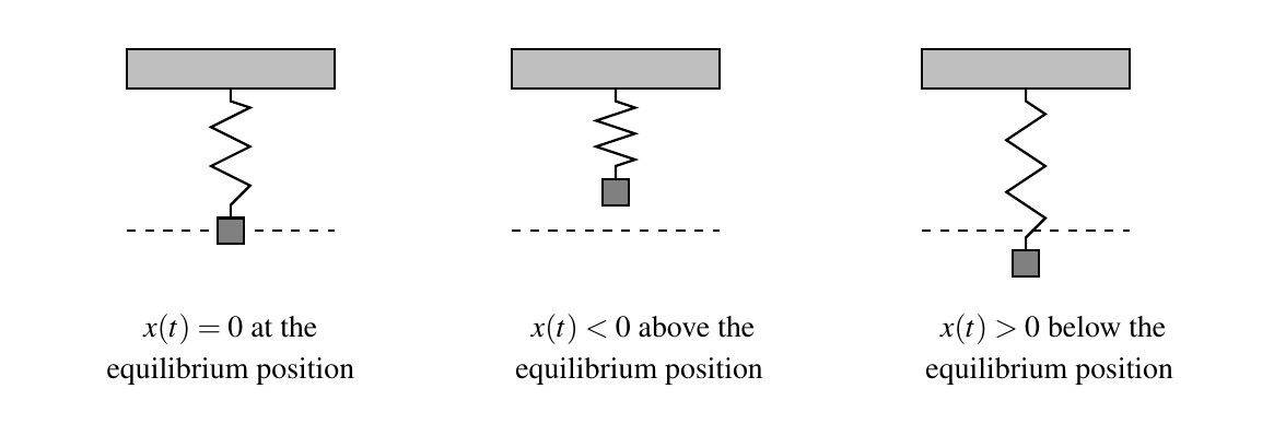
If the object is released above or below the equilibrium position, or if the object is released with an upward or downward velocity, the object will bounce up and down on the end of the spring until some external force stops it. If we let $x(t)$ denote the object’s displacement from the equilibrium position at time $t$ , then $x(t) = 0$ means the object is at the equilibrium position, $x(t) < 0$ means the object is above the equilibrium position, and $x(t) > 0$ means the object is below the equilibrium position. The function $x(t)$ is called the `equation of motion’ of the object.^[12]

If we ignore all other influences on the system except gravity and the spring force, then Physics tells us that gravity and the spring force will battle each other forever and the object will oscillate indefinitely. In this case, we describe the motion as `free’ (meaning there is no external force causing the motion) and `undamped’ (meaning we ignore friction caused by surrounding medium, which in our case is air).

The following theorem, which comes from Differential Equations, gives $x(t)$ as a function of the mass $m$ of the object, the spring constant $k$ , the initial displacement $x_{0}$ of the object and initial velocity $v_{0}$ of the object.

As with $x(t)$ , $x_{0} = 0$ means the object is released from the equilibrium position, $x_{0} < 0$ means the object is released above the equilibrium position and $x_{0}>0$ means the object is released below the equilibrium position. As far as the initial velocity $v_{0}$ is concerned, $v_{0} =0$ means the object is released `from rest,’ $v_{0}<0$ means the object is heading upwards and $v_{0}>0$ means the object is heading downwards.^[13]

Theorem 8.14 Equation for Free Undamped Harmonic Motion

Suppose an object of mass $m$ is suspended from a spring with spring constant $k$ . If the initial displacement from the equilibrium position is $x_{0}$ and the initial velocity of the object is $v_{0}$ , then the displacement $x$ from the equilibrium position at time $t$ is given by $x(t) = A \sin(\omega t + \phi)$ where

$\omega = \sqrt{\dfrac{k}{m}}$ and $A = \sqrt{x_{0}^2 + \left( \dfrac{v_{0}}{\omega}\right)^2}$
$A\sin(\phi) = x_{0}$ and $A\omega\cos(\phi) = v_{0}$

It is a great exercise in `dimensional analysis’ to verify that the formulas given in Theorem 8.14 work out so that $\omega$ has units $\frac{1}{sec}$ and $A$ has units ft. or m, depending on which system we choose.

Example 8.3.5

Example 8.3.5.1

Suppose an object weighing 64 pounds stretches a spring 8 feet.

If the object is attached to the spring and released 3 feet below the equilibrium position from rest, find the equation of motion of the object, $x(t)$ . When does the object first pass through the equilibrium position? Is the object heading upwards or downwards at this instant?

Solution:

In order to use the formulas in Theorem 8.14, we first need to determine the spring constant $k$ and the mass of the object $m$ .

To find $k$ , we use Hooke’s Law $F = kd$ .

We know the object weighs $64$ lbs. and stretches the spring $8$ ft.. Using $F = 64$ and $d = 8$ , we get

$\begin{array}{rcl} 64 &=& k \cdot 8 \\[4pt] k &=& 8 \frac{\text{lbs.}}{\text{ft.}} \end{array}$

To find $m$ , we use $w = mg$ with $w = 64$ lbs. and $g =32 \frac{\text{ft.}}{s^2}$ . We get $m = 2$ slugs.

We can now proceed to apply Theorem 8.14.

If the object is attached to the spring and released 3 feet below the equilibrium position from rest, find the equation of motion of the object, $x(t)$ . When does the object first pass through the equilibrium position? Is the object heading upwards or downwards at this instant?

With $k = 8$ and $m = 2$ , we get $\omega = \sqrt{\frac{k}{m}} = \sqrt{\frac{8}{2}} = 2$ .

Because the object is released 3 feet below the equilibrium position `from rest,’ $x_{0} = 3$ and $v_{0} = 0$ . Therefore, $A = \sqrt{x_{0}^2 + \left( \frac{v_{0}}{\omega}\right)^2} = \sqrt{3^2 + 0^2} = 3$ .

To determine the phase angle, $\phi$ , we have $A\sin(\phi) = x_{0}$ , which in this case gives $3 \sin(\phi) = 3$ so $\sin(\phi) = 1$ . Only $\phi = \frac{\pi}{2}$ and angles coterminal to it satisfy this condition, so we pick^[14] $\phi = \frac{\pi}{2}$ .

Hence, the equation of motion is $x(t) = 3\sin\left(2t + \frac{\pi}{2}\right)$ .

To find when the object passes through the equilibrium position we solve $x(t)= 3\sin\left(2t + \frac{\pi}{2}\right) = 0$ . Going through the usual analysis we find $t = -\frac{\pi}{4} + \frac{\pi}{2} k$ for integers $k$ .

We are interested in the first time the object passes through the equilibrium position, so we look for the smallest positive $t$ value which in this case is $t = \frac{\pi}{4} \approx 0.78$ seconds after the start of the motion.

Common sense suggests that if we release the object below the equilibrium position, the object should be traveling upwards when it first passes through it. To check this answer, we graph one cycle of $x(t)$ . Because our applied domain in this situation is $t \geq 0$ , and the period of $x(t)$ is $T = \frac{2\pi}{\omega} = \frac{2\pi}{2} = \pi$ , we graph $x(t)$ over the interval $[0,\pi]$ . Remembering that $x(t) > 0$ means the object is below the equilibrium position and $x(t) < 0$ means the object is above the equilibrium position, the fact our graph is crossing through the $t$ -axis from positive $x$ to negative $x$ at $t = \frac{\pi}{4}$ confirms our answer.

Rendered by QuickLaTeX.com

Example 8.3.5.2

Suppose an object weighing 64 pounds stretches a spring 8 feet.

If the object is attached to the spring and released 3 feet below the equilibrium position with an upward velocity of $8$ feet per second, find the equation of motion of the object, $x(t)$ . What is the longest distance the object travels above the equilibrium position? When does this first happen? Confirm your result using a graphing utility.

Solution:

In order to use the formulas in Theorem 8.14, we first need to determine the spring constant $k$ and the mass of the object $m$ .

To find $k$ , we use Hooke’s Law $F = kd$ .

We know the object weighs $64$ lbs. and stretches the spring $8$ ft.. Using $F = 64$ and $d = 8$ , we get

$\begin{array}{rcl} 64 &=& k \cdot 8 \\[4pt] k &=& 8 \frac{\text{lbs.}}{\text{ft.}} \end{array}$

To find $m$ , we use $w = mg$ with $w = 64$ lbs. and $g =32 \frac{\text{ft.}}{s^2}$ . We get $m = 2$ slugs.

We can now proceed to apply Theorem 8.14.

If the object is attached to the spring and released 3 feet below the equilibrium position with an upward velocity of $8$ feet per second, find the equation of motion of the object, $x(t)$ . What is the longest distance the object travels above the equilibrium position? When does this first happen? Confirm your result using a graphing utility.

The only difference between this problem and the previous problem is that we now release the object with an upward velocity of $8 \, \frac{\text{ft}}{s}$ . We still have $\omega = 2$ and $x_{0} = 3$ , but now we have $v_{0} = -8$ , the negative indicating the velocity is directed upwards.

Here, we get $A = \sqrt{x_{0}^2 + \left( \frac{v_{0}}{\omega}\right)^2} = \sqrt{3^2 + (-4)^2} = 5$ . From $A\sin(\phi) = x_{0}$ , we get $5\sin(\phi) = 3$ which gives $\sin(\phi) = \frac{3}{5}$ . From $A\omega\cos(\phi) = v_{0}$ , we get $10\cos(\phi) = -8$ , or $\cos(\phi) = -\frac{4}{5}$ .

Hence, $\phi$ is a Quadrant II angle which we can describe in terms of either arcsine or arccosine. The range of arccosine covers Quadrant II, so we choose to express $\phi$ in terms of the arccosine: $\phi = \arccos\left( -\frac{4}{5} \right)$ .

Hence, $x(t)= 5 \sin\left(2t + \arccos\left(-\frac{4}{5}\right) \right)$ .

As the amplitude of $x(t)$ is $5$ , the object will travel at most $5$ feet above the equilibrium position. To find when this happens, we solve the equation $x(t)= 5 \sin\left(2t +\arccos\left( -\frac{4}{5} \right) \right)= -5$ , the negative once again signifying that the object is above the equilibrium position.

Going through the usual machinations, we get $t = -\frac{1}{2} \arccos\left( -\frac{4}{5} \right)-\frac{\pi}{4} + \pi k$ for integers $k$ .

The smallest (positive) of these values occurs when $k=1$ , that is, $t =-\frac{1}{2} \arccos\left( -\frac{4}{5} \right)+ \frac{3\pi}{4} \approx 1.107$ seconds after the start of the motion.

Graphing $x(t) = 5 \sin\left(2t + \arccos\left( -\frac{4}{5} \right) \right)$ , we find the coordinates of the first relative minimum of to be approximately $(1.107,-5).$

Rendered by QuickLaTeX.com

Though beyond the scope of this course, it is possible to model the effects of friction and other external forces acting on the system.^[15]

While we may not have the Physics and Calculus background to derive equations of motion for these scenarios, we can certainly analyze them. We examine three cases in the following example.

Example 8.3.6

Example 8.3.6.1

Write $x(t) = 5e^{-t/5} \cos(t) + 5e^{-t/5} \sqrt{3} \sin(t)$ in the form $x(t) = A(t) \sin(B t + C)$ . Graph $x(t)$ using technology.

Solution:

Write $x(t) = 5e^{-t/5} \cos(t) + 5e^{-t/5} \sqrt{3} \sin(t)$ in the form $x(t) = A(t) \sin(B t + C)$ . Graph $x(t)$ using technology.

We start rewriting $x(t) = 5e^{-t/5} \cos(t) + 5e^{-t/5} \sqrt{3} \sin(t)$ by factoring out $5e^{-t/5}$ from both terms to get $x(t) = 5e^{-t/5} \left( \cos(t) + \sqrt{3} \sin(t)\right)$ . We convert what’s left in parentheses to the required form using the technique introduced in Example 8.2.1 from Section 8.2. We find $\left( \cos(t) + \sqrt{3} \sin(t)\right) = 2\sin\left(t+\frac{\pi}{3}\right)$ so that

$x(t) = 10e^{-t/5} \sin\left(t + \frac{\pi}{3}\right)$

Graphing $x(t)$ reveals some interesting behavior. The sinusoidal nature continues indefinitely, but it is being attenuated. In the sinusoid $A \sin(B t +C)$ , the coefficient $A$ of the sine function is the amplitude. In the case of $x(t) = 10e^{-t/5} \sin\left(t + \frac{\pi}{3}\right)$ , we can think of the function $A(t) = 10e^{-t/5}$ as the amplitude.^[16] As $t \rightarrow \infty$ , $10e^{-t/5} \rightarrow 0$ which means the amplitude shrinks towards zero.

Indeed, if we graph $x = \pm 10e^{-t/5}$ along with $x(t) = 10e^{-t/5} \sin\left(t + \frac{\pi}{3}\right)$ , we see this attenuation taking place with the exponentials acting as a `wave envelope.’

Rendered by QuickLaTeX.com

In this case, the function $x(t)$ corresponds to the motion of an object on a spring where there is a slight force which acts to `damp’, or slow the motion. An example of this kind of force would be the friction of the object against the air. According to this model, the object oscillates forever, but with increasingly smaller and smaller amplitude.

Example 8.3.6.2

Write $x(t) = (t+3)\sqrt{2} \cos(2t) + (t+3) \sqrt{2} \sin(2t)$ in the form $x(t) = A(t) \sin(Bt + C)$ . Graph $x(t)$ using technology.

Solution:

Write $x(t) = (t+3)\sqrt{2} \cos(2t) + (t+3) \sqrt{2} \sin(2t)$ in the form $x(t) = A(t) \sin(Bt + C)$ . Graph $x(t)$ using technology.

Proceeding as in the first example, we factor out $(t+3)\sqrt{2}$ from each term in the function $x(t)$ to get $x(t) = (t+3)\sqrt{2}(\cos(2t) + \sin(2t))$ . We find $(\cos(2t) + \sin(2t)) = \sqrt{2} \sin\left(2t + \frac{\pi}{4}\right)$ , so an equivalent form of $x(t)$ is

$x(t) = 2(t+3) \sin\left(2t + \frac{\pi}{4}\right)$

Graphing $x(t)$ , we find the sinusoid’s amplitude growing. This isn’t too surprising because our amplitude function here is $A(t) = 2(t+3) = 2t+6$ , grows without bound as $t \rightarrow \infty$ .

Rendered by QuickLaTeX.com

The phenomenon illustrated here is `forced’ motion. That is, we imagine that the entire apparatus on which the spring is attached is oscillating as well.

In this particular case, we are witnessing a `resonance’ effect — the frequency of the external oscillation matches the frequency of the motion of the object on the spring. In a mechanical system, this will result in some sort of structural failure.^[17]

Example 8.3.6.3

Compute the period of $x(t) = 5\sin(6t) - 5\sin\left(8t\right)$ . Graph $x(t)$ using technology.

Solution:

Compute the period of $x(t) = 5\sin(6t) - 5\sin\left(8t\right)$ . Graph $x(t)$ using technology.

Last, but not least, we come to $x(t) = 5\sin(6t) - 5\sin(8t)$ . To find the period of this function, we need to determine the length of the smallest interval on which both $f(t) = 5\sin(6t)$ and $g(t) = 5\sin(8t)$ complete a whole number of cycles.

To do this, we take the ratio of their frequencies and reduce to lowest terms: $\frac{6}{8} = \frac{3}{4}$ . This tells us that for every $3$ cycles $f$ makes, $g$ makes $4$ . Hence, the period of $x(t)$ is three times the period of $f(t)$ (which is four times the period of $g(t)$ ), or $\pi$ .

We check our work by graphing $x(t)$ over $[0,\pi]$

The reader may recognize $x(t)$ an example of the `beats’ phenomenon we first saw on Section 8.2.1. Indeed, using a sum to product identity, we may rewrite $x(t)$ as $x(t) = -10 \sin(t) \cos(7t)$ . As we saw in Section 8.2.1 (and Exercises 122 – 125 in Section 8.2), the lower frequency factor, $-10\sin(t)$ determines the `wave-envelope,’ $x = \pm 10 \sin(t)$ .

Rendered by QuickLaTeX.com

This equation of motion also results from `forced’ motion, but here the frequency of the external oscillation is different than that of the object on the spring. The sinusoids here have different frequencies, so they are `out of sync’ and do not amplify each other as in the previous example. Instead, through a combination of constructive and destructive interference, the mass continues to oscillate no more than $10$ units from its equilibrium position indefinitely.

8.3.4 Section Exercises

In Exercises 1 – 20, solve the equation using the techniques discussed in Example 8.3.1 then approximate the solutions which lie in the interval $[0, 2\pi)$ to four decimal places.

$\sin(\theta) = \dfrac{7}{11}$
$\cos(\theta) = -\dfrac{2}{9}$
$\sin(\theta) = -0.569$
$\cos(\theta) = 0.117$
$\sin(\theta) = 0.008$
$\cos(\theta) = \dfrac{359}{360}$
$\tan(t) = 117$
$\cot(t) = -12$
$\sec(t) = \dfrac{3}{2}$
$\csc(t) = -\dfrac{90}{17}$
$\tan(t) = -\sqrt{10}$
$\sin(t) = \dfrac{3}{8}$
$\cos(x) = -\dfrac{7}{16}$
$\tan(x) = 0.03$
$\sin(x) = 0.3502$
$\sin(x) = -0.721$
$\cos(x) = 0.9824$
$\cos(x) = -0.5637$
$\cot(x) = \dfrac{1}{117}$
$\tan(x) = -0.6109$

In Exercises 21 – 38, compute all of the exact solutions of the equation and then list those solutions which are in the interval $[0, 2\pi)$ .

$\sin \left( 5 \theta \right) = 0$
$\cos \left( 3t \right) = \dfrac{1}{2}$
$\sin \left( -2x \right) = \dfrac{\sqrt{3}}{2}$
$\tan \left( 6 \theta \right) = 1$
$\csc \left( 4 t \right) = -1$
$\sec \left( 3x \right) = \sqrt{2}$
$\cot \left( 2 \theta \right) = -\dfrac{\sqrt{3}}{3}$
$\cos \left( 9t \right) = 9$
$\sin \left( \dfrac{x}{3} \right) = \dfrac{\sqrt{2}}{2}$
$\cos \left( \theta+ \dfrac{5\pi}{6} \right) = 0$
$\sin \left( 2t - \dfrac{\pi}{3} \right) = -\dfrac{1}{2}$
$2\cos \left( x + \dfrac{7\pi}{4} \right) = \sqrt{3}$
$\csc( \theta) = 0$
$\tan \left( 2t - \pi \right) = 1$
$\tan^{2} \left( x \right) = 3$
$\sec^{2} \left( \theta \right) = \dfrac{4}{3}$
$\cos^{2} \left( t \right) = \dfrac{1}{2}$
$\sin^{2} \left( x \right) = \dfrac{3}{4}$

In Exercises 39 – 62, solve the equation, giving the exact solutions which lie in $[0, 2\pi)$ .

$\sin \left( \theta \right) = \cos \left( \theta \right)$
$\sin \left( 2t \right) = \sin \left( t \right)$
$\sin \left( 2x \right) = \cos \left( x \right)$
$\cos \left( 2\theta \right) = \sin \left( \theta \right)$
$\cos \left( 2t \right) = \cos \left( t \right)$
$\cos(2x) = 2 - 5\cos(x)$
$3\cos(2 \theta ) + \cos(\theta) + 2 = 0$
$\cos(2t) = 5\sin(t) - 2$
$3\cos(2x) = \sin(x) + 2$
$2\sec^{2}(\theta) = 3 - \tan(\theta)$
$\tan^{2}(t) = 1-\sec(t)$
$\cot^{2}(x) = 3\csc(x) - 3$
$\sec(\theta) = 2\csc(\theta)$
$\cos(t) \csc(t)\cot(t) = 6-\cot^{2}(t)$
$\sin(2x) = \tan(x)$
$\cot^{4}(\theta) = 4\csc^{2}(\theta) - 7$
$\cos(2t) + \csc^{2}(t) = 0$
$\tan^{3} \left( x \right) = 3\tan \left( x \right)$
$\tan^{2} \left( \theta \right) = \dfrac{3}{2} \sec \left( \theta \right)$
$\cos^{3} \left( t \right) = -\cos \left( t \right)$
$\tan (2x) - 2\cos(x) = 0$
$\csc^{3}(\theta) + \csc^{2}(\theta) = 4\csc(\theta) + 4$
$2\tan(t) = 1 - \tan^{2}(t)$
$\tan \left( x \right) = \sec \left( x \right)$

In Exercises 63 – 78, solve the equation, giving the exact solutions which lie in $[0, 2\pi).$

$\sin(6\theta) \cos(\theta) = -\cos(6\theta) \sin(\theta)$
$\sin(3t)\cos(t) = \cos(3t) \sin(t)$
$\cos(2x)\cos(x) + \sin(2x)\sin(x) = 1$
$\cos(5\theta)\cos(3\theta) - \sin(5\theta)\sin(3\theta) = \dfrac{\sqrt{3}}{2}$
$\sin(t) + \cos(t) = 1$
$\sin(x) + \sqrt{3} \cos(x) = 1$
$\sqrt{2} \cos(\theta) - \sqrt{2} \sin(\theta) = 1$
$\sqrt{3} \sin(2t) + \cos(2t) = 1$
$\cos(2x) - \sqrt{3} \sin(2x) = \sqrt{2}$
$3\sqrt{3}\sin(3\theta) - 3\cos(3\theta) = 3\sqrt{3}$
$\cos(3t) = \cos(5t)$
$\cos(4x) = \cos(2x)$
$\sin(5\theta) = \sin(3\theta)$
$\cos(5t) = -\cos(2t)$
$\sin(6x) + \sin(x) = 0$
$\tan(x) = \cos(x)$

In Exercises 79 – 88, solve the equation.

$\arccos(2x) = \pi$
$\pi - 2\arcsin(t) = 2\pi$
$4\arctan(3x-1)-\pi=0$
$6 \, \text{arccot}(2t) - 5\pi = 0$
$4 \,\text{arcsec}\left(\frac{x}{2}\right) = \pi$
$12 \,\text{arccsc}\left(\frac{t}{3}\right) = 2\pi$
$9 \arcsin^{2}(x) - \pi^2 = 0$
$9 \arccos^{2}(t) - \pi^2 = 0$
$8 \, \text{arccot}^{2}(x)+3\pi^2=10 \pi \, \text{arccot}(x)$
$6 \arctan(t)^2= \pi \arctan(x)+\pi^2$
(a) With the help of your classmates, determine the number of solutions to $\sin(x) = \frac{1}{2}$ in $[0,2\pi)$ . Then find the number of solutions to $\sin(2x) = \frac{1}{2}$ , $\sin(3x) = \frac{1}{2}$ and $\sin(4x) = \frac{1}{2}$ in $[0,2\pi)$ . What pattern emerges? Explain how this pattern would help you solve equations like $\sin(11x) = \frac{1}{2}$ .
(b) Repeat the above exercise focusing on $\sin\left(\frac{x}{2}\right) = \frac{1}{2}$ , $\sin\left(\frac{3x}{2}\right) = \frac{1}{2}$ and $\sin\left(\frac{5x}{2}\right) = \frac{1}{2}$ . What pattern emerges here?
(c) Replace sine with tangent and $\frac{1}{2}$ with $1$ and repeat the whole exploration.
Suppose an object weighing pounds is suspended from the ceiling by a spring which stretches feet to its equilibrium position when the object is attached.
1. Find the spring constant $k$ in $\frac{\text{lbs.}}{\text{ft.}}$ and the mass of the object in slugs.
2. Find the equation of motion of the object if it is released from $1$ foot below the equilibrium position from rest. When is the first time the object passes through the equilibrium position? In which direction is it heading?
3. Find the equation of motion of the object if it is released from $6$ inches above the equilibrium position with a downward velocity of $2$ feet per second. Find when the object passes through the equilibrium position heading downwards for the third time.

Section 8.3 Exercise Answers can be found in the Appendix … Coming soon

Don't forget to divide the $2\pi k$ by $3$ as well! ↵
On many calculators, there is no function button for cotangent. In that case, we would use the quotient identity and graph $y = \frac{\cos(3t)}{\sin(3t)}$ instead. The reader is invited to see what happens if we would graph $y= \frac{1}{\tan(3t)}$ instead. ↵
Note that we do not list $\theta = 2\pi$ as part of the solution over the interval $[0,2\pi)$ because $2\pi$ is not in $[0, 2\pi)$ . ↵
See Section 0.5.5 for a review of this concept. ↵
We invite the reader to try the `polynomial approach' used in the previous problem to see what difficulties are encountered. ↵
A product equaling zero means, necessarily, one or both factors is 0. See Section 0.1.1. ↵
As always, when in doubt, write it out! ↵
We've seen how squaring both sides can lead to extraneous solutions in Section 0.2 and Chapter 4. Here, squaring both sides admits an entire family of extraneous solutions. ↵
Well, assuming the object isn't subjected to relativistic speeds $\dots$ ↵
This is a consequence of Newton's Second Law of Motion $F = ma$ where $F$ is force, $m$ is mass and $a$ is acceleration. In our present setting, the force involved is weight which is caused by the acceleration due to gravity. ↵
Note that $1$ pound $= 1 \, \frac{\text{slug foot}}{\text{second}^2}$ and 1 Newton $= 1 \, \frac{\text{kg meter}}{\text{second}^2}$ . ↵
To keep units compatible, if we are using the English system, we use feet (ft.) to measure displacement. If we are in the SI system, we measure displacement in meters (m). Time is always measured in seconds (s). ↵
The sign conventions here are carried over from Physics. If not for the spring, the object would fall towards the ground, which is the `natural' or `positive' direction. Because the spring force acts in direct opposition to gravity, any movement upwards is considered `negative'. ↵
For confirmation, we note that $A\omega\cos(\phi) = v_{0}$ , which in this case reduces to $6\cos(\phi) = 0$ . ↵
Take a good Differential Equations class to see this! ↵
This is the same sort of phenomenon we saw in Section 8.2.1. ↵
The reader is invited to investigate the destructive implications of resonance. ↵